
Published on July 30, 2024 9:11 PM GMT

Background
Sparse autoencoders recover a diversity of interpretable, monosemantic features, but present an intractable problem of scale to human labelers. We investigate different techniques for generating and scoring text explanations of SAE features.
Key Findings
- Open source models generate and evaluate text explanations of SAE features reasonably well, albeit somewhat worse than closed models like Claude 3.5 Sonnet.Explanations found by LLMs are similar to explanations found by humans.Automatically interpreting 1.5M features of GPT-2 with the current pipeline would cost $1300 in API calls to Llama 3.1 or $8500 with Claude 3.5 Sonnet. Prior methods cost ~$200k with Claude.Code can be found at https://github.com/EleutherAI/sae-auto-interp.We built a small dashboard to explore explanations and their scores: https://cadentj.github.io/demo/
Generating Explanations
Sparse autoencoders decompose activations into a sum of sparse feature directions. We leverage language models to generate explanations for activating text examples. Prior work prompts language models with token sequences that activate MLP neurons (Bills et al. 2023), by showing the model a list of tokens followed by their respective activations, separated by a tab, and listed one per line.
We instead highlight max activating tokens in each example with a set of <<delimiters>>. Optionally, we choose a threshold of the example’s max activation for which tokens are highlighted. This helps the model distinguish important information for some densely activating features.
Example 1: and he was <<over the moon>> to findExample 2: we'll be laughing <<till the cows come home>>! ProExample 3: thought Scotland was boring, but really there's more <<than meets the eye>>! I'dWe experiment with several methods for augmenting the explanation. Full prompts are available here.
Chain of thought improves general reasoning capabilities in language models. We few-shot the model with several examples of a thought process that mimics a human approach to generating explanations. We expect that verbalizing thought might capture richer relations between tokens and context.
Step 1. List a couple activating and contextual tokens you find interesting. Search for patterns in these tokens, if there are any.- The activating tokens are all parts of common idioms.- The previous tokens have nothing in common.Step 2. Write down general shared features of the text examples.- The examples contain common idioms.- In some examples, the activating tokens are followed by an exclamation mark.- The text examples all convey positive sentiment.Step 3. List the tokens that the neuron boosts in the next token predictionSimilar tokens: "elated", "joyful", "thrilled".- The top logits list contains words that are strongly associated with positive emotions.Step 4. Generate an explanation[EXPLANATION]: Common idioms in text conveying positive sentiment.Activations distinguish which sentences are more representative of a feature. We provide the magnitude of activating tokens after each example.
We compute the logit weights for each feature through the path expansion where
is the model unembed and
is the decoder direction for a specific feature. The top promoted tokens capture a feature’s causal effects which are useful for sharpening explanations. This method is equivalent to the logit lens (nostalgebraist 2020); future work might apply variants that reveal other causal information (Belrose et al. 2023; Gandelsman et al. 2024).
Scoring explanations
Text explanations represent interpretable “concepts” in natural language. How do we evaluate the faithfulness of explanations to the concepts actually contained in SAE features?
We view the explanation as a classifier which predicts whether a feature is present in a context. An explanation should have high recall – identifying most activating text – as well as high precision – distinguishing between activating and non-activating text.
Consider a feature which activates on the word “stop” after “don’t” or “won’t” (Gao et al. 2024). There are two failure modes:
- The explanation could be too broad, identifying the feature as activating on the word “stop”. It would have high recall on held out text, but low precision.The explanation could be too narrow, stating the feature activates on the word “stop” only after “don’t”. This would have high precision, but low recall.
One approach to scoring explanations is “simulation scoring”(Bills et al. 2023) which uses a language model to assign an activation to each token in a text, then measures the correlation between predicted and real activations. This method is biased toward recall; given a broad explanation, the simulator could mark the token “stop” in every context and still achieve high correlation.
We experiment with different methods for evaluating the precision and recall of SAE features.
Detection
Rather than producing a prediction at each token, we ask a language model to identify whether whole sequences contain a feature. Detection is an “easier”, more in-distribution task than simulation: it requires fewer few-shot examples, fewer input/output tokens, and smaller, faster models can provide reliable scores. We can scalably evaluate many more text examples from a wider distribution of activations. Specifically, for each feature we draw five activating examples from deciles of the activation distribution and twenty random, non-activating examples. We then show a random mix of 5 of those examples and ask the model to directly say which examples activate given a certain explanation.
Fuzzing
We investigate fuzzing, a closer approximation to simulation than detection. It’s similar to detection, but activating tokens are <<delimited>> in each example. We prompt the language model to identify which examples are correctly marked. Like fuzzing from automated software testing, this method captures specific vulnerabilities in an explanation. Evaluating an explanation on both detection and fuzzing can identify whether a model is classifying examples for the correct reason.
We draw seven activating examples from deciles of the activation distribution. For each decile, we mark five correctly and two incorrectly for a total of seventy examples. To “incorrectly” mark an example, we choose N non activating tokens to delimit where N is the average number of marked tokens across all examples. Not only are detection and fuzzing scalable to many examples, but they’re also easier for models to understand. Less capable – but faster – models can provide reliable scores for explanations.
Future work might explore more principled ways of creating ‘incorrectly fuzzed’ examples. Ideally, fuzzing should be an inexpensive method of generating counterexamples directly from activating text. For example:
- Replacing activating tokens with non-activating synonyms to check if explanations that identify specific token groups are precise enough.Replacing semantically relevant context with a masked language model before delimiting could determine if explanations are too context dependent.
Generation
We provide a language model an explanation and ask it to generate sequences that contain the feature. Explanations are scored by the number of activating examples a model can generate. However, generation could miss modes of a feature’s activation distribution. Consider the broad explanation for “stop”. A generator might only write counterexamples that contain “don’t” but miss occurrences of “stop” after “won’t”.
Neighbors
The above methods face similar issues to simulation scoring: they are biased toward recall, and counterexamples sampled at random are a weak signal for precision. As we scale SAEs and features become sparser and more specific, the inadequacy of recall becomes more severe (Gao et al. 2024)
Motivated by the phenomenon of feature splitting (Bricken et al. 2023), we use “similar” features to test whether explanations are precise enough to distinguish between similar contexts. We use cosine similarity between decoder directions of features to find counterexamples for an explanation. Our current approach does not thoroughly account for co-occurrence of features, so we leave those results in the appendix.
Future work will investigate using neighbors as an important mechanism to make explanations more precise. Other methods for generating counterexamples, such as exploring RoBERTa embeddings of explanations, could be interesting as well.
Results
We conduct most of our experiments using detection and fuzzing as a point of comparison. Both metrics are inexpensive and scalable while still providing a clear picture of feature patterns and quality.
We envision an automated interpretability pipeline that uses cheap and scalable methods to map out relevant features, supplemented by more expensive, detailed techniques. One could start with self-interpreted features (Chen et al 2024, Ghandeharioun et al. 2024), quickly find disagreements with our pipeline, then apply interpretability agents (Rott Shaham et al. 2024) to hone in on a true explanation.
Llama-3 70b is used as an explainer and scorer except where explicitly mentioned.
Explainers
How does the explainer model size affect explanation quality?
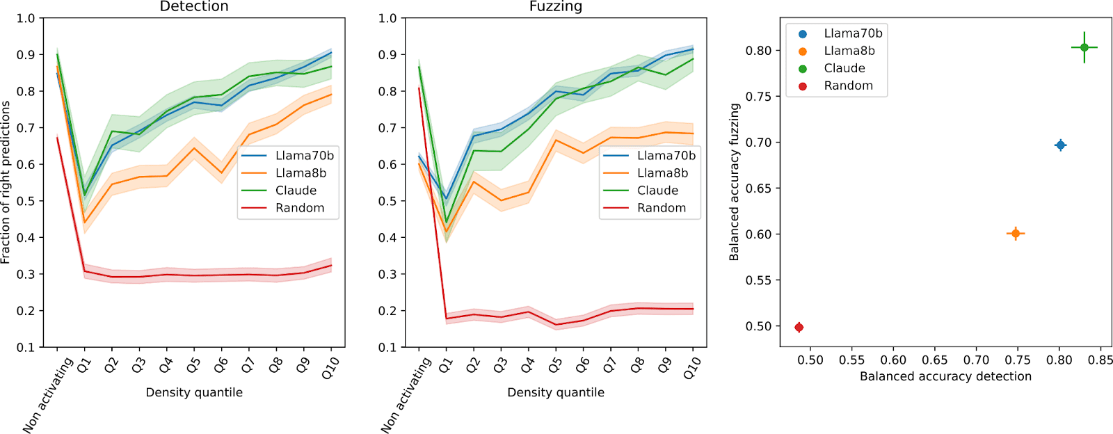
We evaluate model scale and human performance on explanation quality using the 132k latent GPT-2 top-K SAEs. Models generate explanations for 350 features while a human (Gonçalo) evaluates thirty five. Manual labeling is less scalable and wider error bars reflect this fact.
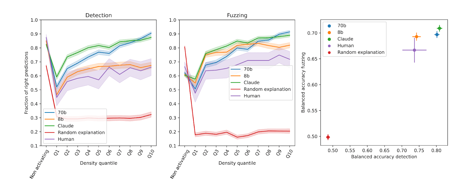
As a comparison, we show the performance of a scorer that is given a random explanation for the features. As expected, better models generate better explanations. We want to highlight that explanations given by humans are not always optimizing for high fuzzing and detection scores, and that explanations that humans find good could require different scoring metrics. We discuss this further in the text.
Providing more information to the explainer
A human trying to interpret a feature on Neuronpedia might incorporate various statistics before providing an explanation. We experiment with giving the explainer different information to understand whether this improves performance.
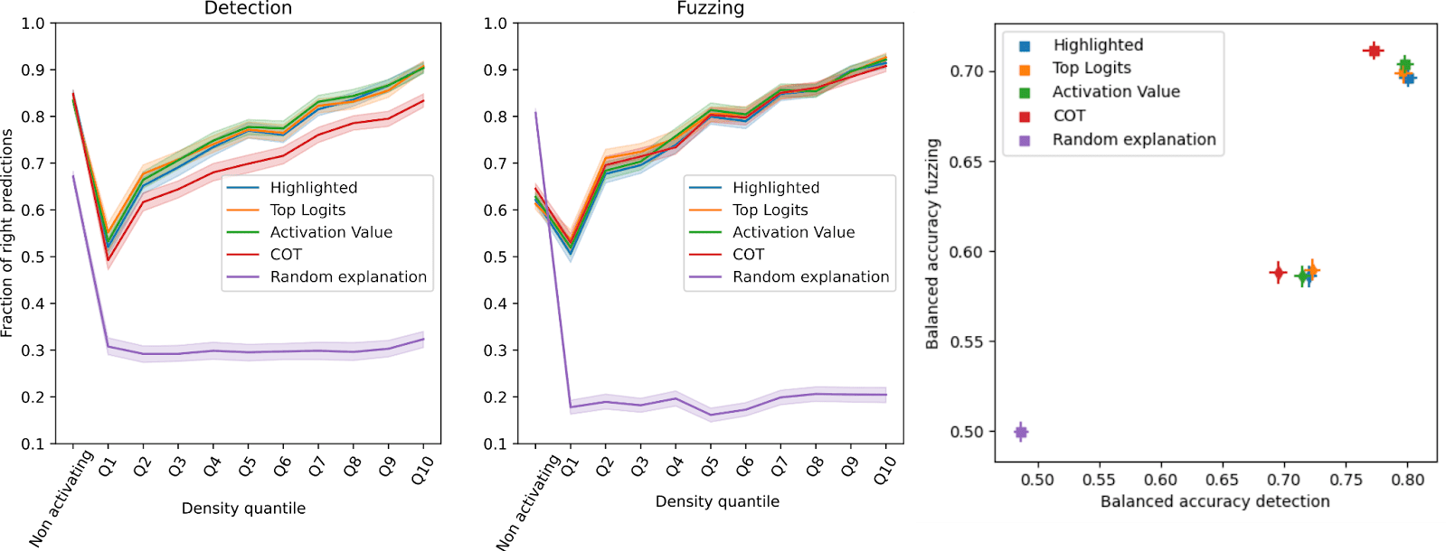
Providing more information to the explainer does not significantly improve scores for both GPT-2 (squares) and Llama-3 8b (diamonds) SAEs. Instead, models tend to overthink and focus on extraneous information, leading to vague explanations. This could be due to the quantization and model scale.
Giving the explainer different samples of top activating examples
Bricken et al. use forty nine examples from different quantiles of the activation distribution for generating explanations. We analyze how varying the number of examples and sampling from different portions of the top activations affects explanation quality.
- Top activating examples: The top ten, twenty, or forty examplesSampling from top examples: Twenty or forty examples sampled from the top 200 examplesSampling from all examples: Ten, twenty, or forty examples sampled randomly from all examplesA mixture: Twenty examples from the top 200 plus twenty examples sampled from all examples
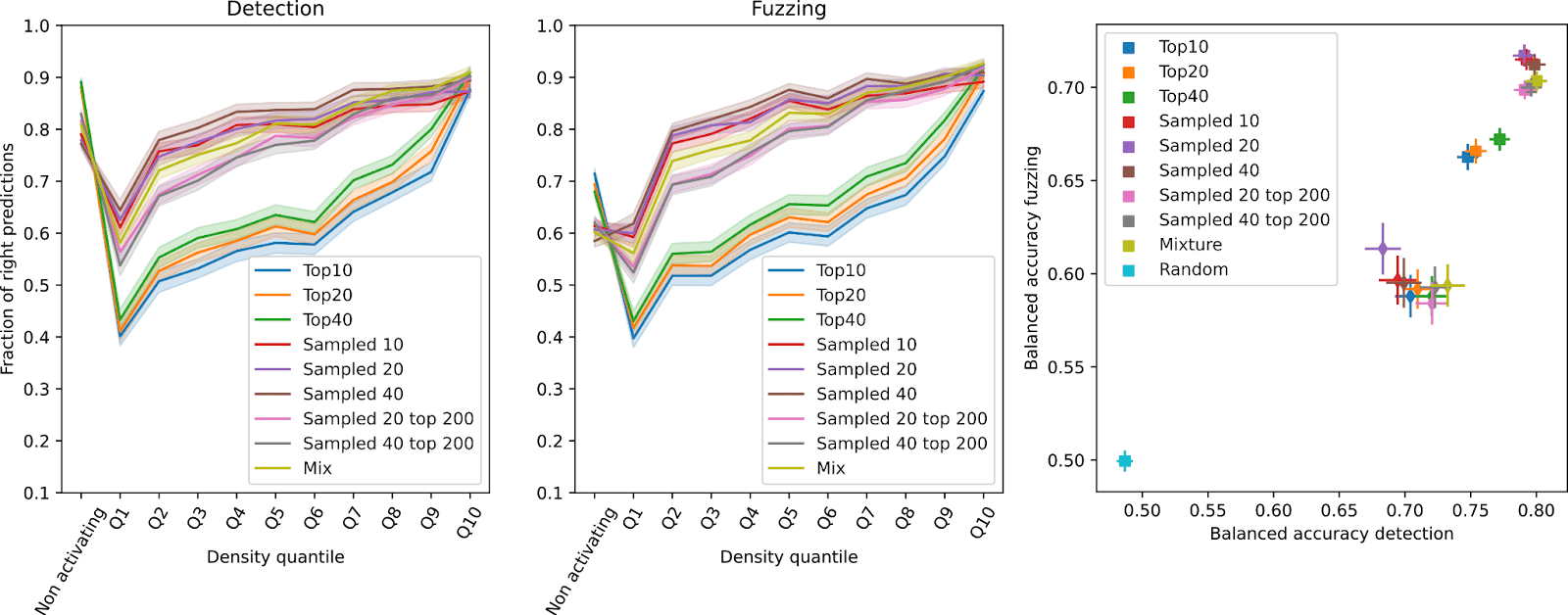
Sampling from the top N examples produces narrow explanations that don’t capture behavior across the whole distribution. Instead, sampling evenly from all examples produces explanations that are robust to less activating examples. This makes sense – matching the train and test distribution should lead to higher scores. Anecdotally, however, randomly sampling examples in coarser SAEs may make explanations worse due to more diverse text examples at different quantiles.
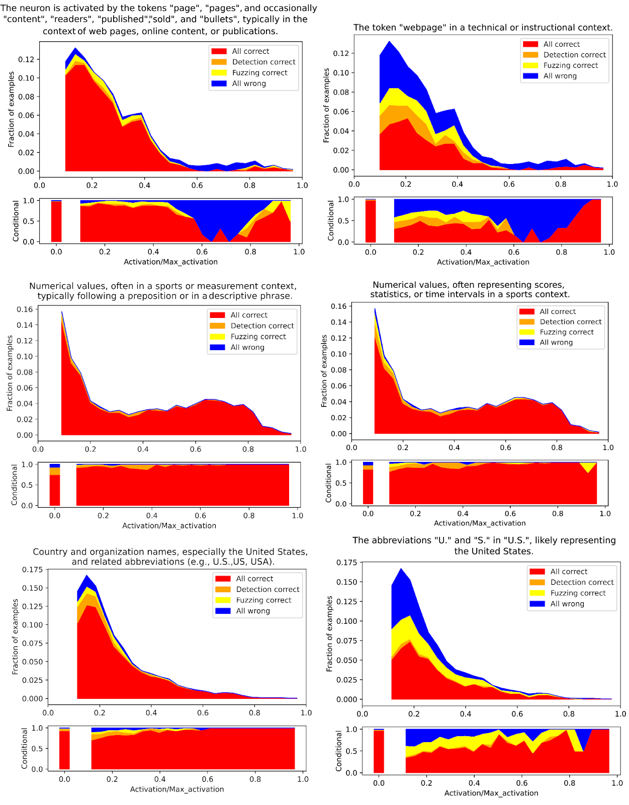
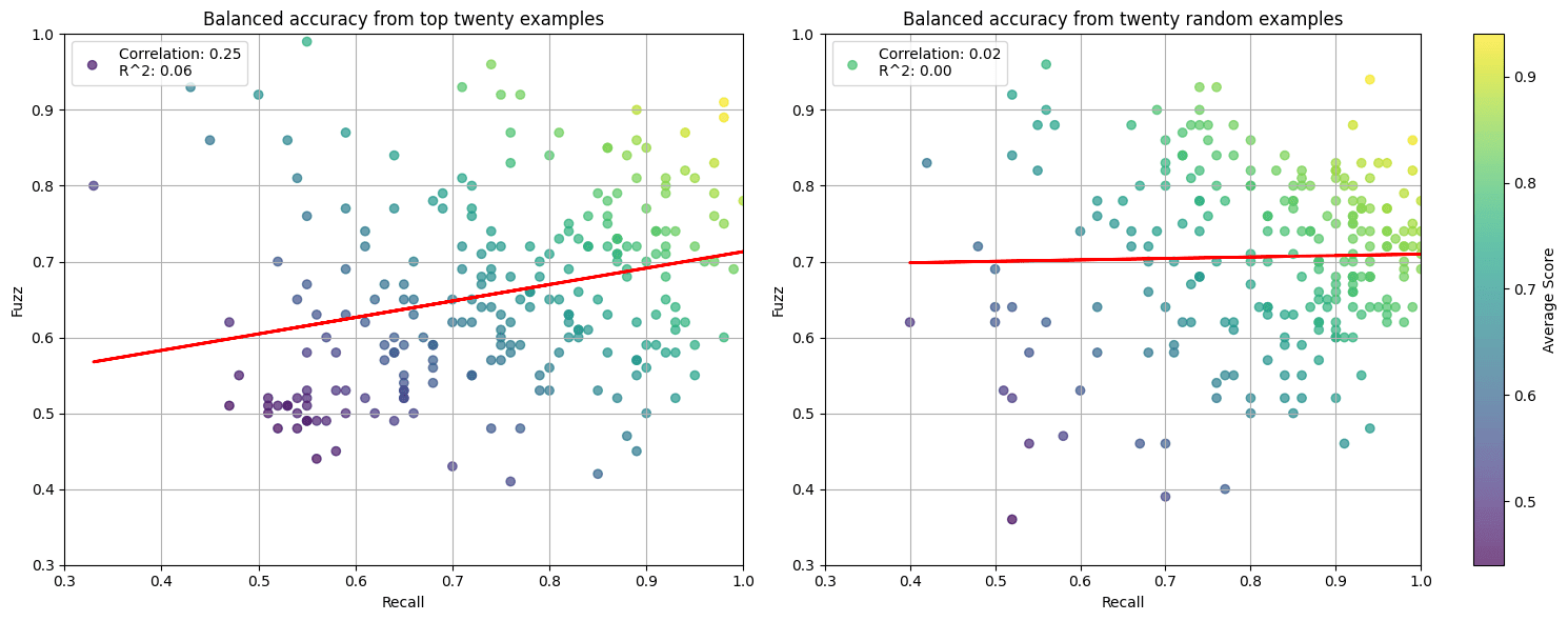
Visualizing activation distributions
We can visualize explanation quality across the whole distribution of examples. In the figures below, we evaluate 1,000 examples with fuzzing and detection. We compare explanations generated from the whole distribution (left column) versus explanations generated from the top N examples (right column). Explanations “generalize” better when the model is presented with a wider array of examples.
Scorers
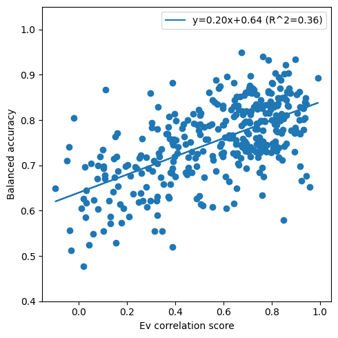
How do methods correlate with simulation?
The average balanced accuracy of detection and fuzzing correlates with the simulation scoring proposed by Bills et al. (Pearson correlation of 0.61). We do not view simulation scoring as a “ground-truth” score, but we feel that this comparison is an important sanity check since we expect our proposed methods to correlate reasonably with simulation.
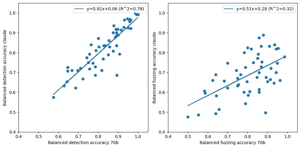
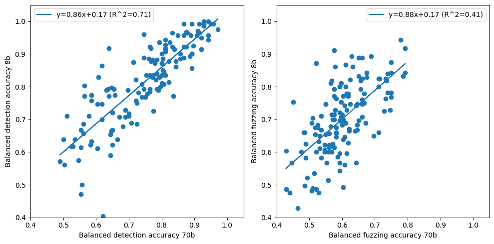
How does scorer model size affect scores?
We see that both detection and fuzzing scoring are affected by the size of the evaluator model, even when given the same explanation. Still we observe that scores correlate across model size; one could estimate some calibration curve given more evaluator explanations.
What do detection and fuzzing distinctly reveal?
On the surface, detection and fuzzing appear quite similar. We plot their correlation on two sampling methods to understand where they diverge. You can find an interactive version of the plots here.
Ideally, fuzzing tests whether explanations are precise enough to separate activating tokens from irrelevant context. On manual inspection of features, we find detection and fuzzing largely agree on activating examples. However, fuzzing utterly fails to classify mislabeled examples. We hypothesize that the task may be too hard which is concerning given that fuzzed examples have tokens selected at random. Future work could measure the effect of more few-shot examples and model performance.
How precise is detection and fuzzing scoring without adversarial examples?
We prompt the language model to generate ten sentences at high temperature that activate a given explanation. A significant fraction of explanations aren’t precise enough to generate activating examples, possibly due to model size or the failure of explanations at identifying critical context. We’d like to scale generation scoring in future work to better understand how model scale/biases affect scoring quality and whether generation is a reliable signal of precision.
How much more scalable is detection/fuzzing?
| Method | Prompt Tokens | Unique Prompt Tokens | Output Tokens | Runtime in seconds |
| Explanation | 397 | 566.45 ± 26.18 | 29.90 ± 7.27 | 3.14 ± 0.48 |
| Detection/Fuzzing | 725 | 53.13 ± 10.53 | 11.99 ± 0.13 | 4.29 ± 0.14 |
| Simulation | – | 24074.85 ± 71.45 | 1598.1 ± 74.9 | 73.9063 ± 13.5540 * |
We measure token I/O and runtime for explanation and scoring. For scoring methods, these metrics correspond to the number of tokens/runtime to evaluate five examples. Tests are run on a single NVIDIA RTX A6000 on a quantized Llama-3 70b with VLLM prefix caching. Simulation scoring is notably slower as we used Outlines (a structured generation backend) to enforce valid JSON responses.
| Method | Prompt Tokens | Output Tokens | GPT 4o mini | Claude 3.5 Sonnet |
| Explanation | 963.45 | 29.90 | 160 $ | 3400 $ |
| Detection/Fuzzing | 778.13 | 11.99 | 125 $ | 2540 $ |
| Simulation | 24074.85 | 1598.1 | 4700 $ | 96K $ |
Prices as of publishing date, July 30, 2024, on the OpenRouter API, per million features.
Filtering with known heuristics
Automated interpretability pipelines might involve a preprocessing step that filters out features for which there are known heuristics. We demonstrate a couple simple methods for filtering out context independent unigram features and positional features.
Positional Features
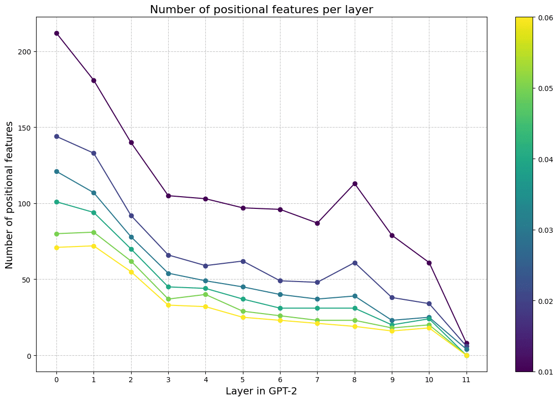
Some neurons activate on absolute position rather than on specific tokens or context. We cache activation frequencies for each feature over the entire context length of GPT2 and filter for features with high mutual information with position (Voita et. al 2023).
Similar to Voita et al. 2023, we find that earlier layers have a higher number of positional features, but that these features represent a small fraction (<0.1%) of all features of any given layer.
Unigram features
Some features activate on tokens independent of the surrounding context. We filter for features which have twenty or fewer unique tokens among the top eighty percent of their activations. To verify that these features are context independent, we create sentences with 19 tokens randomly sampled from the vocabulary plus a token that activates the feature.
We do this twice per token in the unique set, generating upwards of forty scrambled examples per feature. We run the batch through the autoencoder and measure the fraction of scrambled sentences with nonzero activations.
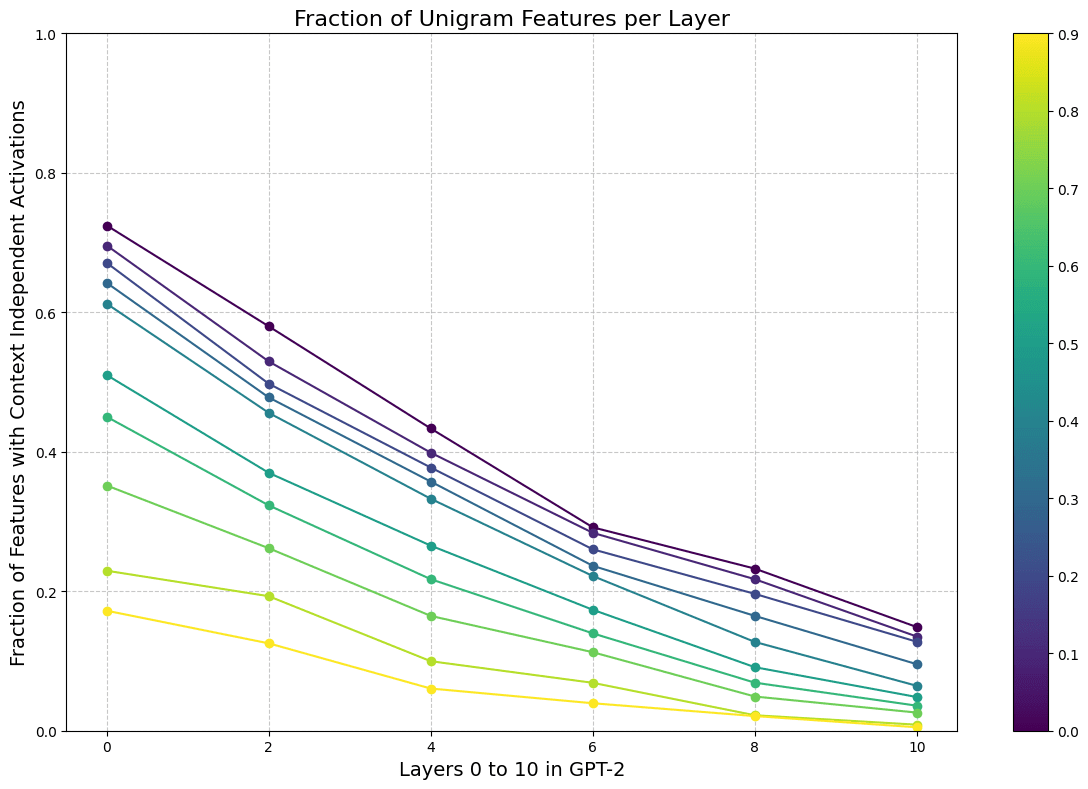
We analyze a random sample of 1k features from odd layers in GPT-2. Earlier layers have a substantial portion of context independent features.
Some features also activate following specific tokens. Instead of saving features with twenty or fewer activating tokens, we search for features with <= twenty unique prior tokens. This process only yields a handful of features in our sample.
Sparse Feature Circuits
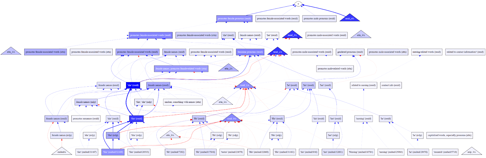
Figure 12: A sparse feature circuit for a classifier on the bias in bios task with manual labels on each node.
We demonstrate our automated interpretability pipeline by explaining and scoring all features in the Bias in Bios classifier task from the Sparse Feature Circuits paper (Marks et al 2024). We CoT prompt LLama-3 70b to generate an explanation given a feature’s top logits and activations (above 70% the max activation). Explanations are scored with detection and fuzzing. A full dashboard is available here.
Some features cannot be explained from their activation patterns
Toward the end of the circuit [L4_12420, ATTN3_2959], features activate on dense sets of unrelated tokens. Note Llama’s initial confusion at providing an explanation for L4_12420.
ACTIVATING TOKENS: Various function words and punctuation marks.PREVIOUS TOKENS: No interesting patterns.Step 1.- The activating tokens are mostly function words (prepositions, conjunctions, auxiliary verbs) and punctuation marks.- The previous tokens have nothing in common.Luckily, the top logits provide some signal. Llama picks up on this and correctly revises its explanation to include the information.
(Part 2)SIMILAR TOKENS: [' her', ' she', ' herself', ' She', ' hers', 'she', ' Her', 'She', 'Her', 'her'].- The top logits list suggests a focus on pronouns related to a female subject.Many features like L4_12420 promote and suppress certain sets of tokens (Bloom and Lin 24, Bricken et al. 23). We consider two broad categorizations.
Input features activate in response to certain patterns of the sequence. Early layers of the BiB circuit contain many of such type which activate on pronouns [MLP0_2955] or gendered names [RESID1_9877].
Output features have interpretable casual effects on model predictions. Consider late layers which sharpen the token distribution [Lad et al 24] and induction heads [Olsson et al 22] which match and copy patterns of the sequence. Respective features in Pythia [4_30220, ATTN2_27472] are uninterpretable from activation patterns but promote sets of semantically related tokens.
Features that represent intermediate model computation are incompatible with methods that directly explain features from properties of the input. Consider the true explanation for L4_12420: “this feature promotes gendered pronouns”. Given the explanation, our scorer must predict whether the original model (Pythia) would promote a gendered pronoun given a set of prior tokens. Casual scoring methods are necessary for faithfully evaluating these explanations (Huang et al. 23).
Further, the distinction between these two groups is blurry. Features that appear as “input features” might have important causal effects that our explainer cannot capture. Future work might investigate ways to automatically filter for causal features at scale.
Future Directions
More work on scoring
Generation scoring seems promising. Some variations we didn’t try include:
- Asking a model to generate counterexamples for classification. This is hard as models aren’t great at consistently generating negations or sequences that almost contain a concept.Using BERT to find sentences with similar embeddings or perform masked language modeling on various parts of the context, similar to fuzzing.
Human evaluation of generated examples
Neuronpedia is set to upload the GPT-2 SAEs we have looked at. We plan to upload our results so people can red-team and evaluate the explanations provided by our auto-interp pipeline. For now we have a small dashboard which allows people to explore explanations and their scores.
More work on generating explanations.
To generate better and more precise explanations we may add more information to the context of the explaining model, like results of the effects of ablation, correlated tokens and other information that humans use to try to come up with new explanations. We may also incentivize the explainer model to hill-climb a scoring objective by iteratively showing it the explanations generated, their scores and novel examples.
Acknowledgements
We would like to thank Joseph Bloom, Sam Marks, Can Rager, Jannik Brinkmann and Sam Marks for their comments and suggestions, and to Neel Nanda, Sarah Schwettmann and Jacob Steinhardt for their discussion.
Contributions
Caden Juang wrote most of the code and devised the methods and framework. Caden did the experiments related to feature sorting and Sparse Feature Circuits. Gonçalo Paulo ran the experiments and analysis related to explanation and scoring, including hand labeling a set of random features. Caden and Gonçalo wrote up the post. Nora Belrose supervised, reviewed the manuscript and trained the Llama 3 8b SAEs. Jacob Drori designed many of the prompts and initial ideas. Sam Marks suggested the framing for input/output features in the SFC section.
Appendix
Neighbor scoring
We experiment with neighbor scoring, a variant of detection where we sample the top ten activating examples from the ten nearest neighbors by cosine similarity.
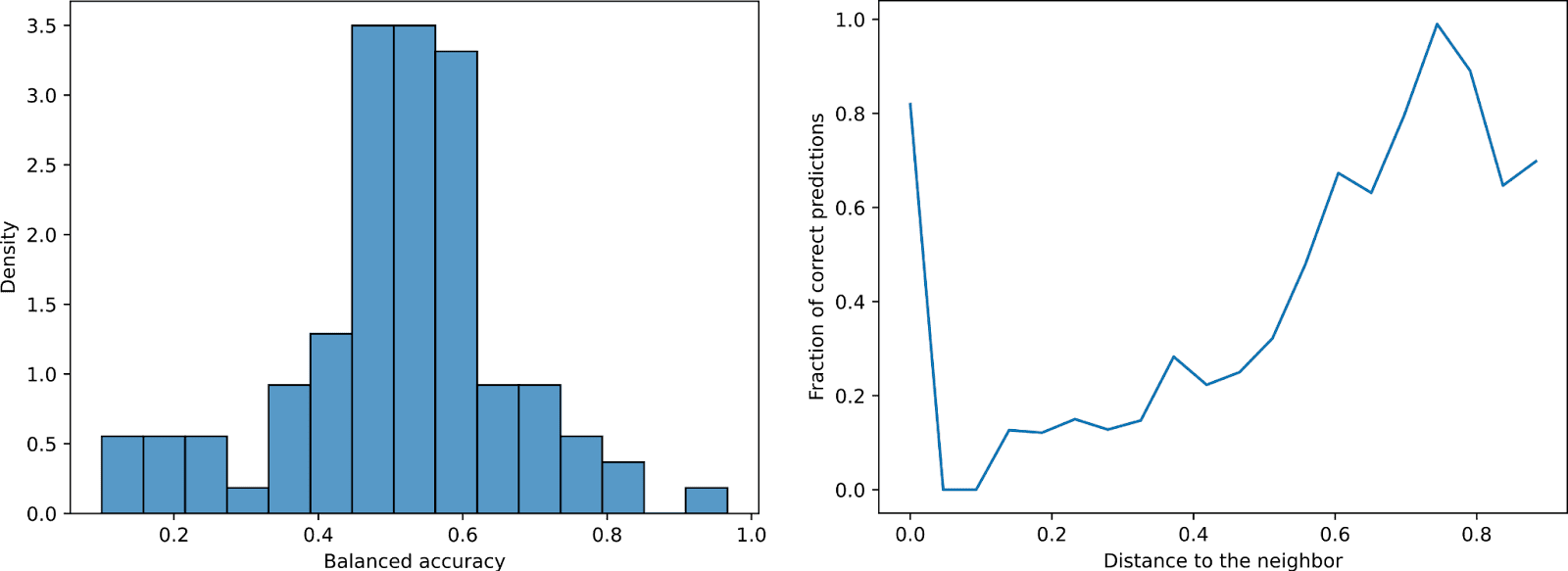
Figure S1: (Left) Balanced accuracy of detection when provided examples from neighboring features as non activating examples. The balanced accuracy drops from > 80% to ~random, indicating that the explanations generated are not specific enough to distinguish very similar contexts. (Right) As the neighbor distance increases, the scorer’s accuracy increases.
We find that explanations are not precise enough to differentiate between semantically similar counterexamples. However, this isn’t entirely the scorer’s fault. Similar features often co-occur on the same examples (Bussman et al. 24) which we do not filter for. We leave methods for scalably checking co-occurrence to future work. We think neighbor scoring is an effective solution as dictionaries become sparser and features more specific.
Random Directions
Formal Grammars for Autointerp
Perhaps automated interpretability using natural language is too unreliable. With a bunch of known heuristics for SAE features, maybe we can generate a domain specific language for explanations, and use in-context learning or fine tuning to generate explanations using that grammar, which could potentially be used by an external verifier.
<explanation> ::= “Activates on ” <subject> [“ in the context of ” <context>]<subject> ::= <is-plural> | <token><is-plural> ::= “the tokens ” | “the token ”<token> ::= ( a generated token or set of related tokens )<context> ::= ( etc. )The (loose) grammar above defines explanations like: “Activates on the token pizza in the context of crust”.
Debate
We imagine a debate setup where each debater is presented with the same, shuffled set of examples. Each debater has access to a scratchpad and a quote tool. Thoughts in the scratchpad are hidden from the judge which is instructed to only accept verified quotes (Khan et al. 24). After a bout of reasoning, the debaters present an opening argument consisting of three direct, verified quotes and an explanation sampled at high temperature.
1. Quote One2. Quote Two3. Quote ThreeExplanation: ...The “arguments” and explanations from N debaters are passed to a weaker judge model without access to chain of thought or the original text. The judge chooses the top explanation from presented arguments.
Discuss
