本文详细介绍了如何使用WordStat和QDA Miner构建一个自动机器学习文档分类（AML-DC）模型，用于快速、可重复、可靠和可审计地将大量调查结果分类为正面和负面情感类别。文章以2016年共和党初选辩论的推特数据为例，详细阐述了数据预处理、模型构建、模型应用等步骤，并展示了模型的性能评估结果。通过该案例，读者可以了解AML-DC模型的构建过程和应用场景，并学习如何使用WordStat和QDA Miner工具进行文本分析和分类。

🤔 **数据预处理：**文章首先对共和党初选辩论的推特数据集进行了预处理，包括筛选出正负面情感的推文，并随机抽取一部分作为样本数据，剩余数据用于模型训练。同时，将训练数据划分为正负面两个子集，用于构建分类模型。

📊 **模型构建：**文章使用WordStat工具构建了AML-DC模型，尝试了朴素贝叶斯和K近邻算法，最终选择了K (2)-Nearest Neighbour模型，并使用了逆文档频率（IDF）特征加权，该模型在平均精确率、平均召回率和准确率方面表现出色，达到97%以上。

🔍 **模型应用：**文章使用构建好的AML-DC模型，在QDA Miner中对样本数据进行自动编码，预测样本数据的正负面情感类别，并通过混淆矩阵评估模型性能。

📈 **结果分析：**模型成功编码了464个样本，其中84.7%被预测为负面情感，15.3%被预测为正面情感。文章还展示了混淆矩阵、特征选择、邻近图、多维尺度分析等文本分析方法，帮助读者理解模型结果。

💡 **工具应用：**文章详细介绍了WordStat和QDA Miner这两个工具在AML-DC模型构建和应用中的具体操作步骤，包括数据导入、模型参数设置、结果分析等，为读者提供了实践指导。

INTRODUCTION

Part I of our blog series introduced Automatic Machine Learning Document Classification (AML-DC).

Part II of our blog series on Automatic Machine Learning Document Classification (AML-DC) provides a practical and detailed walkthrough on the development and implementation of a supervised AML-DC model in fast, reproducible, reliable and auditable way.

RESEARCH PROBLEM

How does one classify a large corpora of survey results into positive and negative sentiment classes, in a fast, reproducible, reliable and auditable way?

METHOD

Our solution to the research problem was to first built a AML-DC model in WordStat and then used QDA Miner to auto-encode the large corpora of survey results with negative and positive sentiment classes.

For this blog, we accessed the “First GOP debate sentiment analysis” dataset. The GOP dataset contains tens of thousands of tweets about the early 2016 August GOP debate in Ohio. The authors had asked contributors to do both sentiment analysis and data categorization. Contributors were asked if the tweet was relevant, which candidate was mentioned, what subject was mentioned, and then what the sentiment was for a given tweet.  Non-relevant messages were removed from the uploaded dataset.

Data preparation stage

The GOP dataset was pre-processed in R Studio,  as detailed below:

We accessed the unit-level, GOP dataset (13,871 rows by 20 columns). Data variables kept for this study were:
ID: unique identification code for each case;TEXT: Text containing GOP comments recorded for each person; andSENTIMENT LABEL: neutral, negative and positive sentiments.
We filtered the data and saved the positive sentiments and negative sentiments a single file – called this the MAIN FILE. Notice we deleted all neutral sentiment cases (3,142 rows).We randomly selected a 5 percent sample of both positive and negative cases from the MAIN FILE and striped-off their sentiment labels – called this the SAMPLER FILE, (536rows).We built some model learning datasets from the MAIN FILE after excluding the cases in the SAMPLER FILE and saved them in separate files:

Positive sentiments (2,130 rows) – called this the POSITIVE FILE; andNegative sentiments (8,063 rows) – called this the NEGATIVE FILE.

Note the sample size imbalance between positive and negative learning datasets.

Data preparation stage in WordStat and QDA

Creating separate QDA Miner / WordStat projects.

In this section we imported csv files created in R Studio into QDA Miner/WordStat and saved them as separate projects (i.e. Positive.ppj , Negative.ppj and Sampler.ppj). Below are the steps we followed to process these projects.

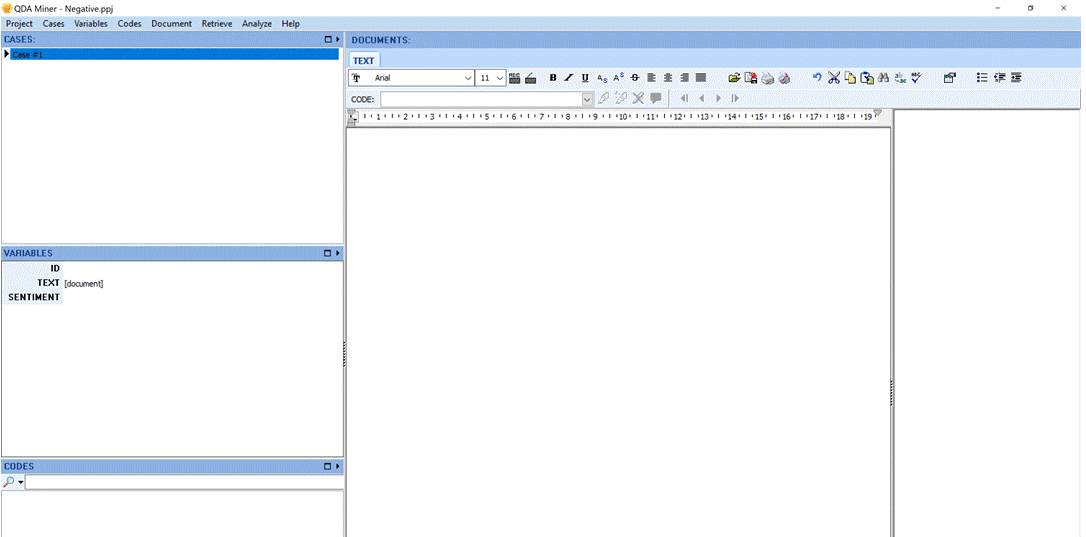
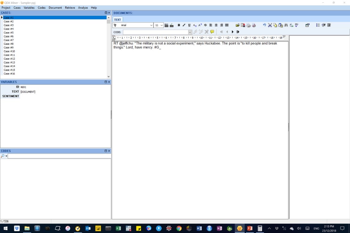
We created QDA Miner project templates in hold these data variables: ID, Text and Sentiment (label). Below is an image of a QDA Miner template for negative sentiment documents.

Figure 1: Template for negative sentiment documents

Importing sentiment documents into the QDA Miner/WordStat projects

We imported the respective cases into their QDA Miner/WordStat projects, as shown below for the negative sentiment documents (i.e. the NEGATIVE FILE). We repeated the process for the positive sentiment documents (i.e. the NEGATIVE FILE) and for the sample sentiment documents (i.e. the SAMPLER FILE).

Figure 2: Importing negative sentiment documents into WordStat – step 1 of 2.

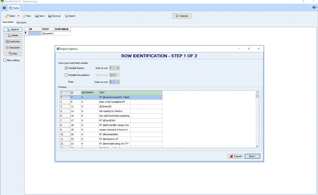
Figure 3: Importing negative sentiment documents into WordStat – step 2 of 2.

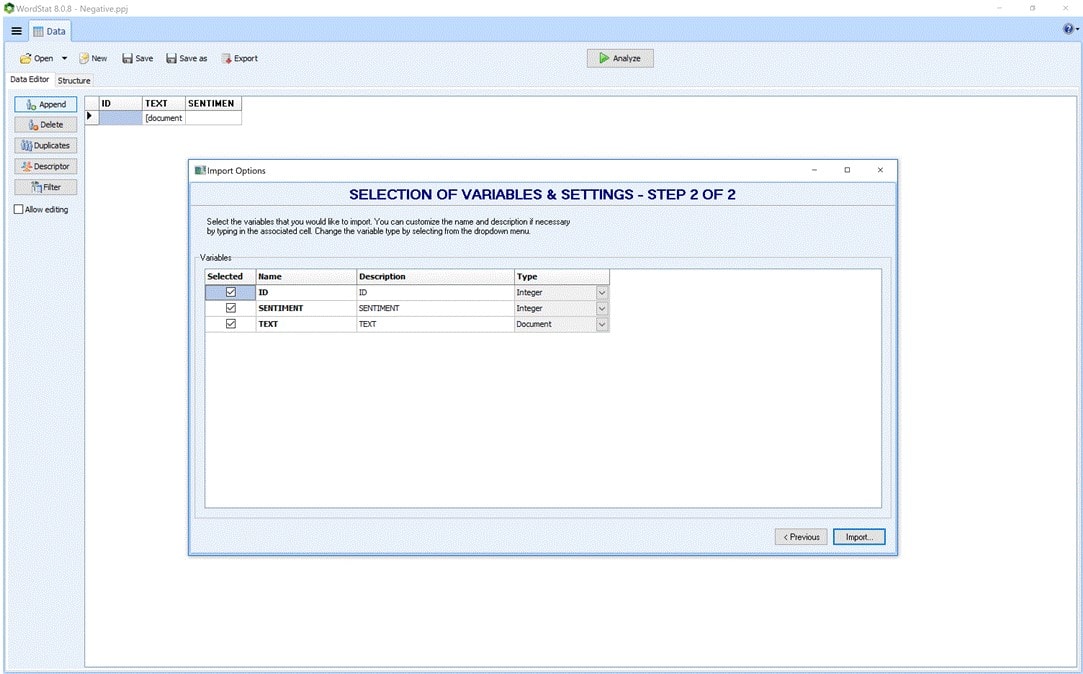
Figure 4: Appending negative sentiment documents in WordStat.

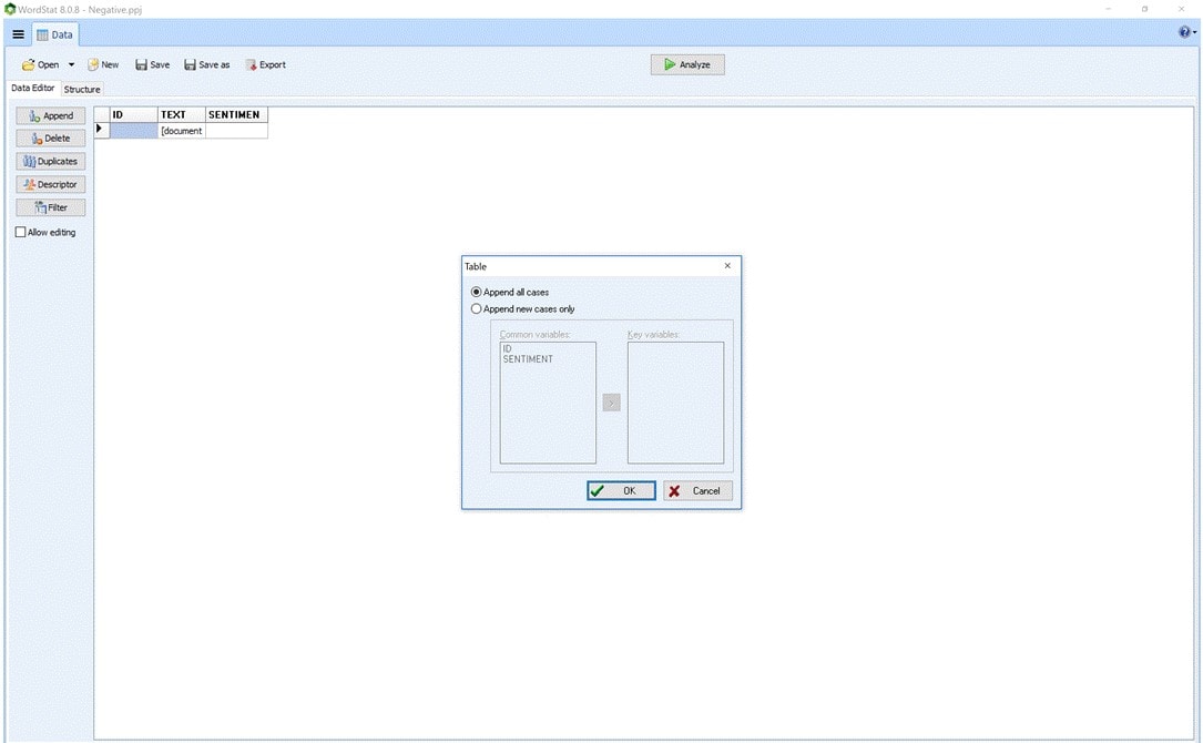
Figure 5: Imported negative sentiment documents in WordStat.

Figure 6: Imported positive sentiment documents in WordStat.

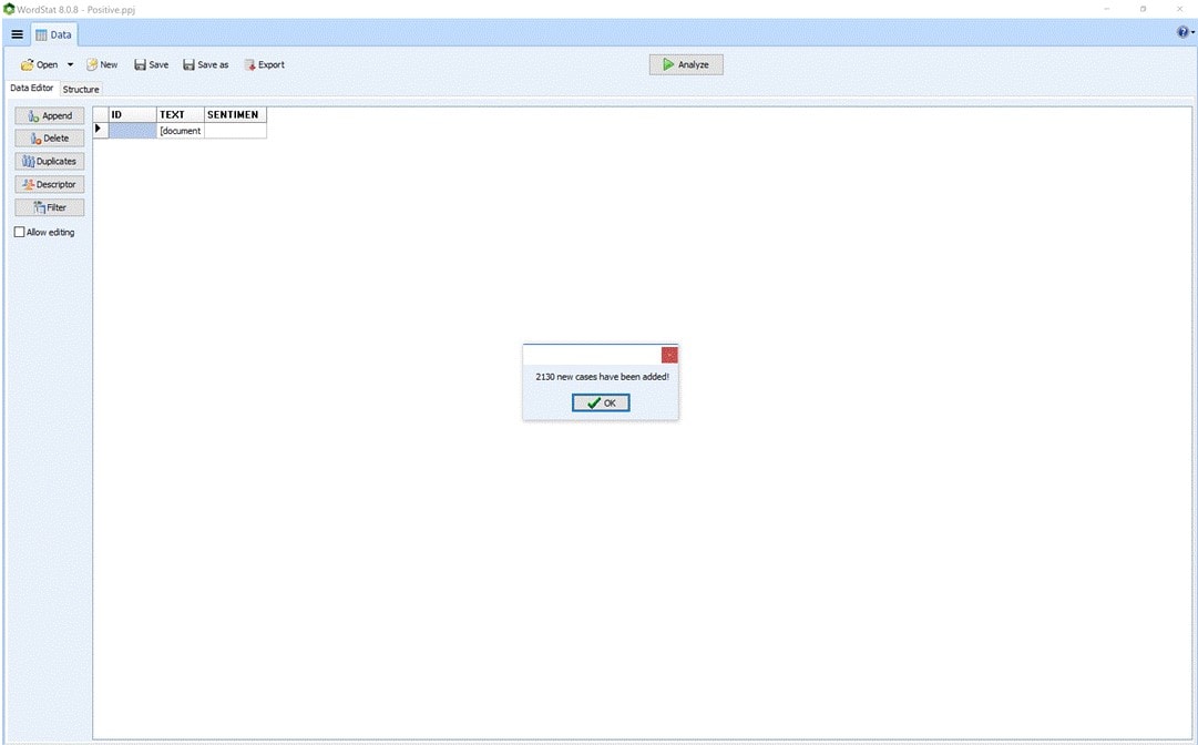
Figure 7: Imported Sample(r) sentiment documents in WordStat.

Building the WordStat AM-CL model

We concatenated the WordStat projects with the positive and negative sentiment corpora and saved them as single WordStat project, shown below.

Figure 8: The Positive and Negative sentiment documents in WordStat.

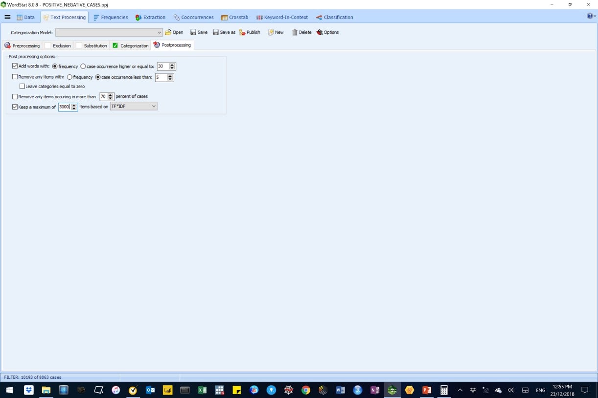
We selected the pre-and post-processing parameters for the WordStat AM-CL model as shown in the next two images, below. 

Figure 9: Pre-processing parameters used in the WordStat AM-CL model.

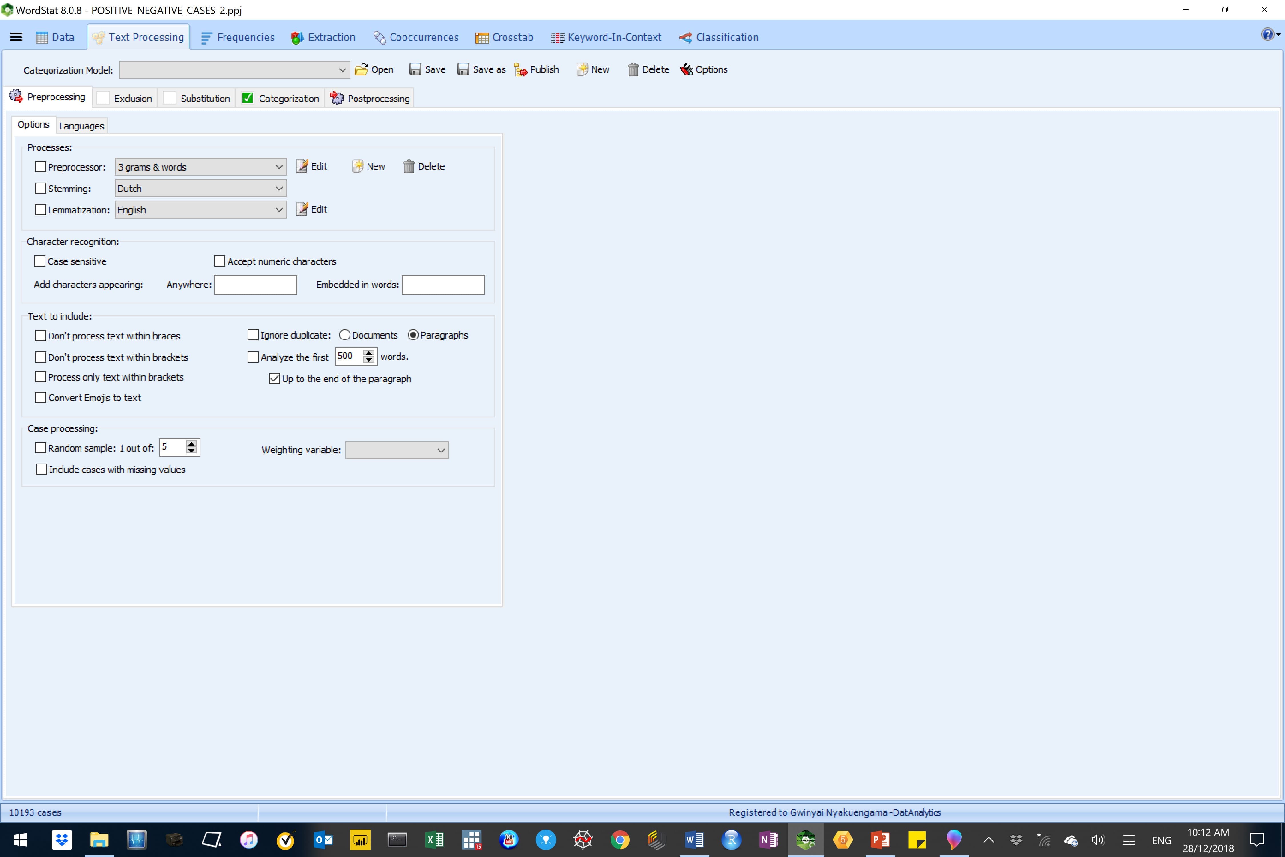
Figure 10: Post-processing parameters used in the WordStat AM-CL model.

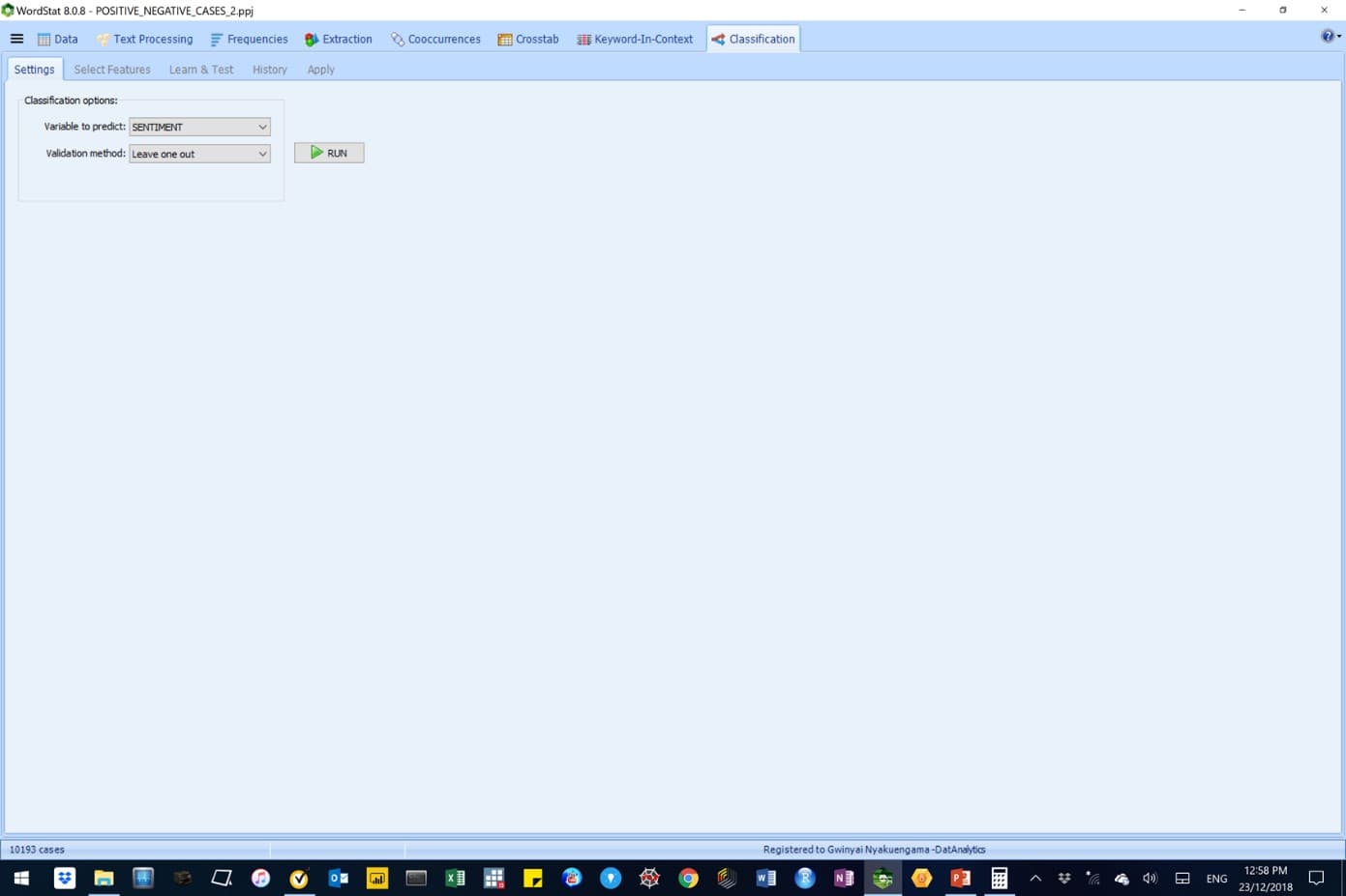
We ran our AM-CL classification model, under the Classification tab, to predict sentiment using the ‘leave‑one‑out’ validation method, as shown below.

Figure 10: Classification options for the WordStat AM-CL model.

RESULTS

We experimented with the Naïve Bayes and the K-Nearest Neighbour (k-NN) learning algorithms to build the AM-CL model which we used to predict case-occurrence for sentiments.

Below are outputs from those modelling experiments.

We ultimately, settled for a K (2)-Nearest Neighbour AM-CL model, which employed the Inverse Document Frequency (or IDF) feature weighting. We selected this model because of its superior model performance parameters namely, average precision (98%), average recall (97%), nominal and ordinary accuracy (98%).

For details on machine learning and terminology used here please refer to Part I of our blog series on Automatic Machine Learning Document Classification (AML-DC) in Nyakuengama (2019).

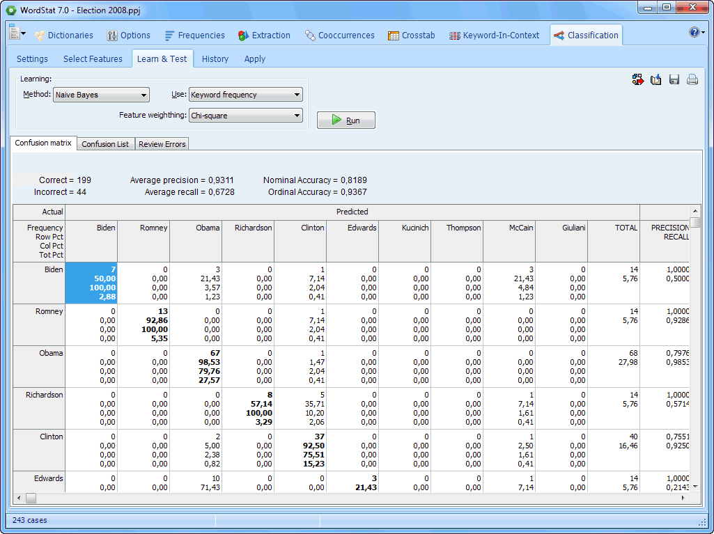
Figure 10: A Naïve Bayes AM-CL model in WordStat.

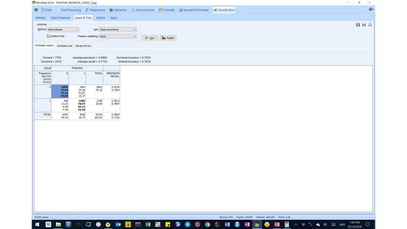
Figure 11: A K (30)-Nearest Neighbour AM-CL model in WordStat

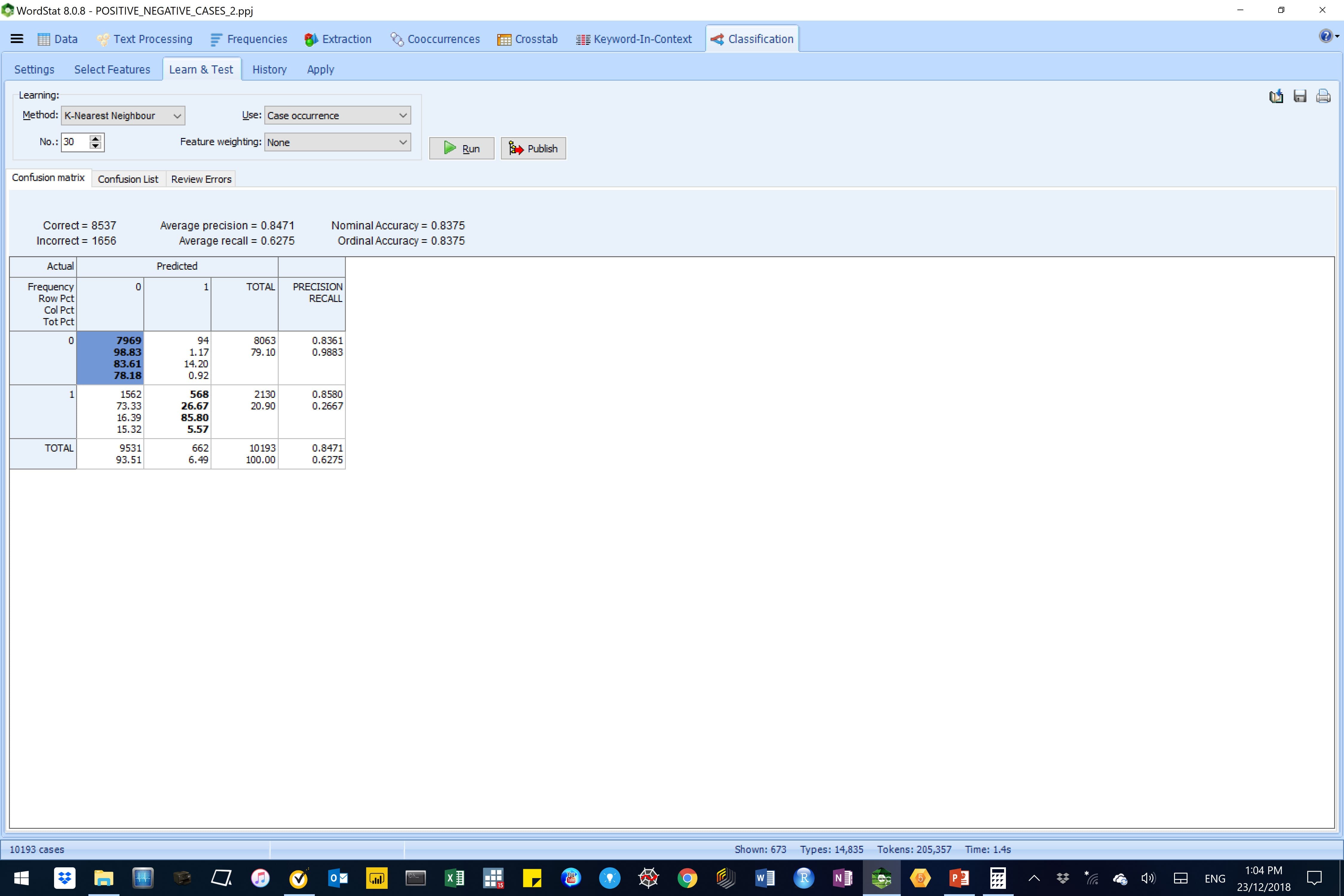
Figure 11: A K (3)-Nearest Neighbour AM-CL model in WordStat, without feature weighting

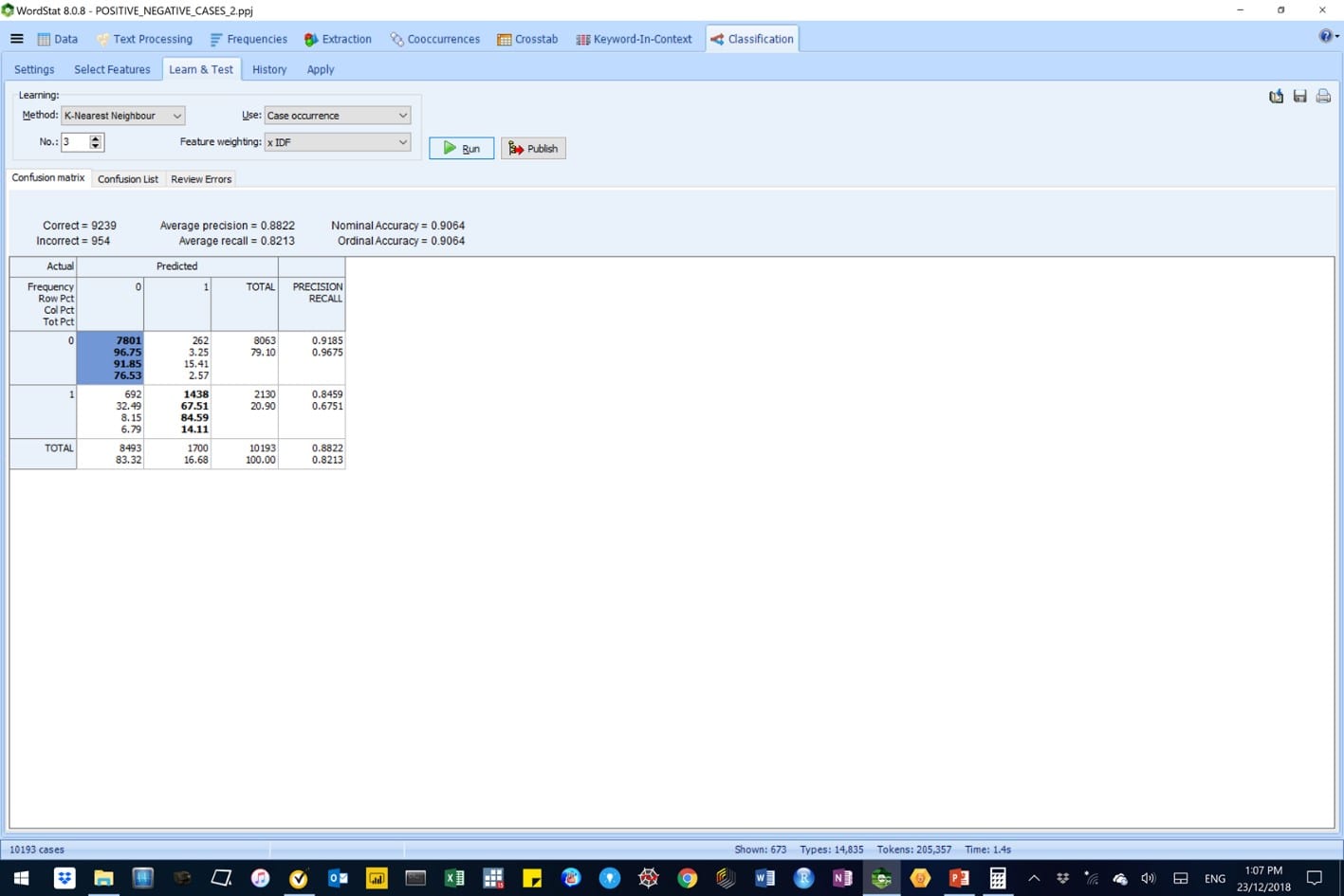
Figure 12: A K (3)-Nearest Neighbour AM-CL model in WordStat, with Inverse Document Frequency (IDF) feature weighting

Figure 12: A K (2)-Nearest Neighbor AM-CL model in WordStat, with Inverse Document Frequency (IDF) feature weighting is the selected model.

Applying the WordStat AML-DC model using QDA Miner

In this section we applied the AML-DC model on the Sample(r) project created in WordStat, above.

The overall objective was to use the AML-DC model to auto-encode unknown sentiments in cases contained in the WordStat Sample(r) project.

Below are a series of illustrational images.

Firstly, we opened the WordStat Sample(r) project with a total of 536 cases with unknown sentiment classes.

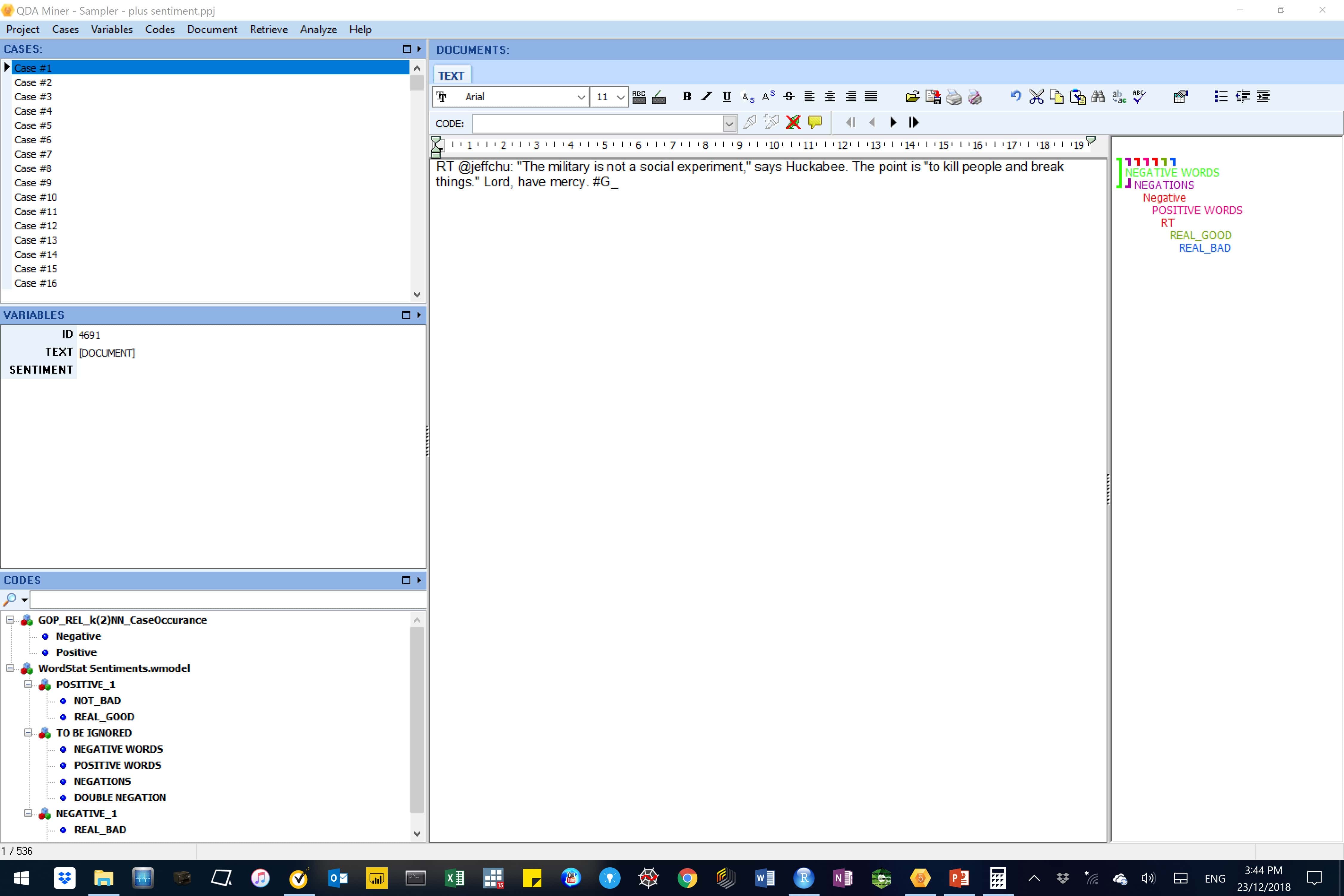
Figure 13: This image shows the sentiment documents in the WordStat Sample(r) project.

Secondly, we retrieved text in the WordStat Sample (r) project (as shown in the next series of related images).

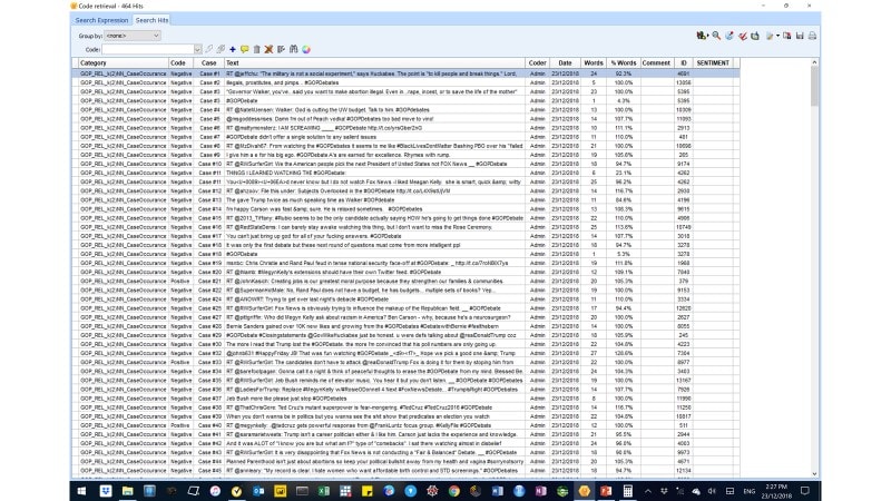
Figure 14: Text retrieval of paragraphs from sentiment documents contained in the WordStat Sample(r) project.

Figure 15: Text retrieval of paragraphs from sentiment documents contained in the WordStat Sample(r) project – with the ‘show/hide automatic document classification panel’ button activated (yellow highlight).

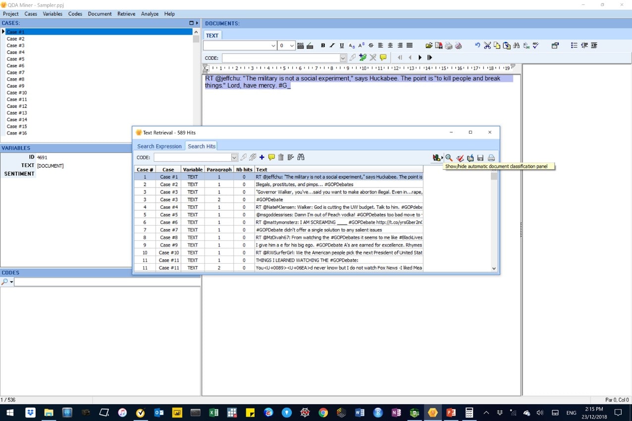
Figure 16: Selection of the WordStat automatic document classification model (GOP_REL_k(2)NN_CaseOccurance) which will be used to auto-encode individual cases in sentiment documents contained in the WordStat Sample(r) project.

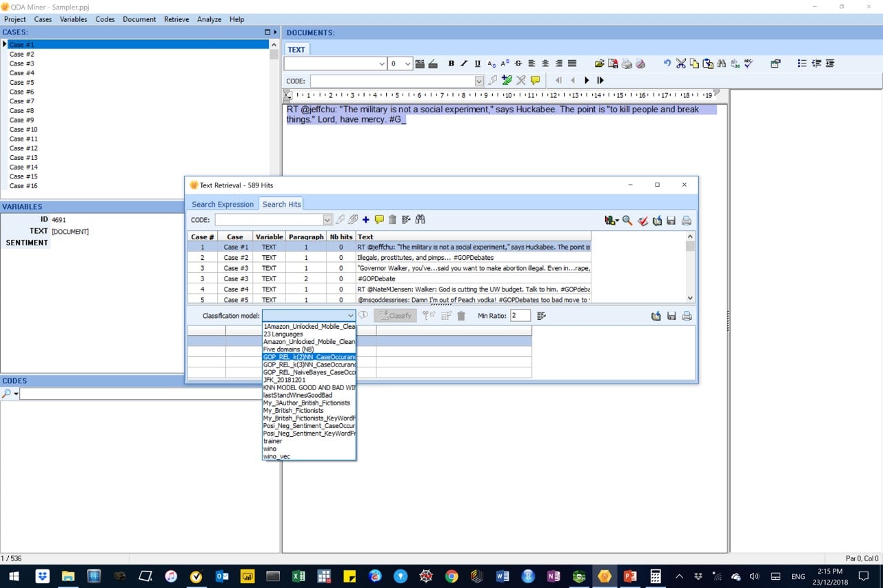
Figure 17: In this image, the “Perform automatic classification” button is highlighted.

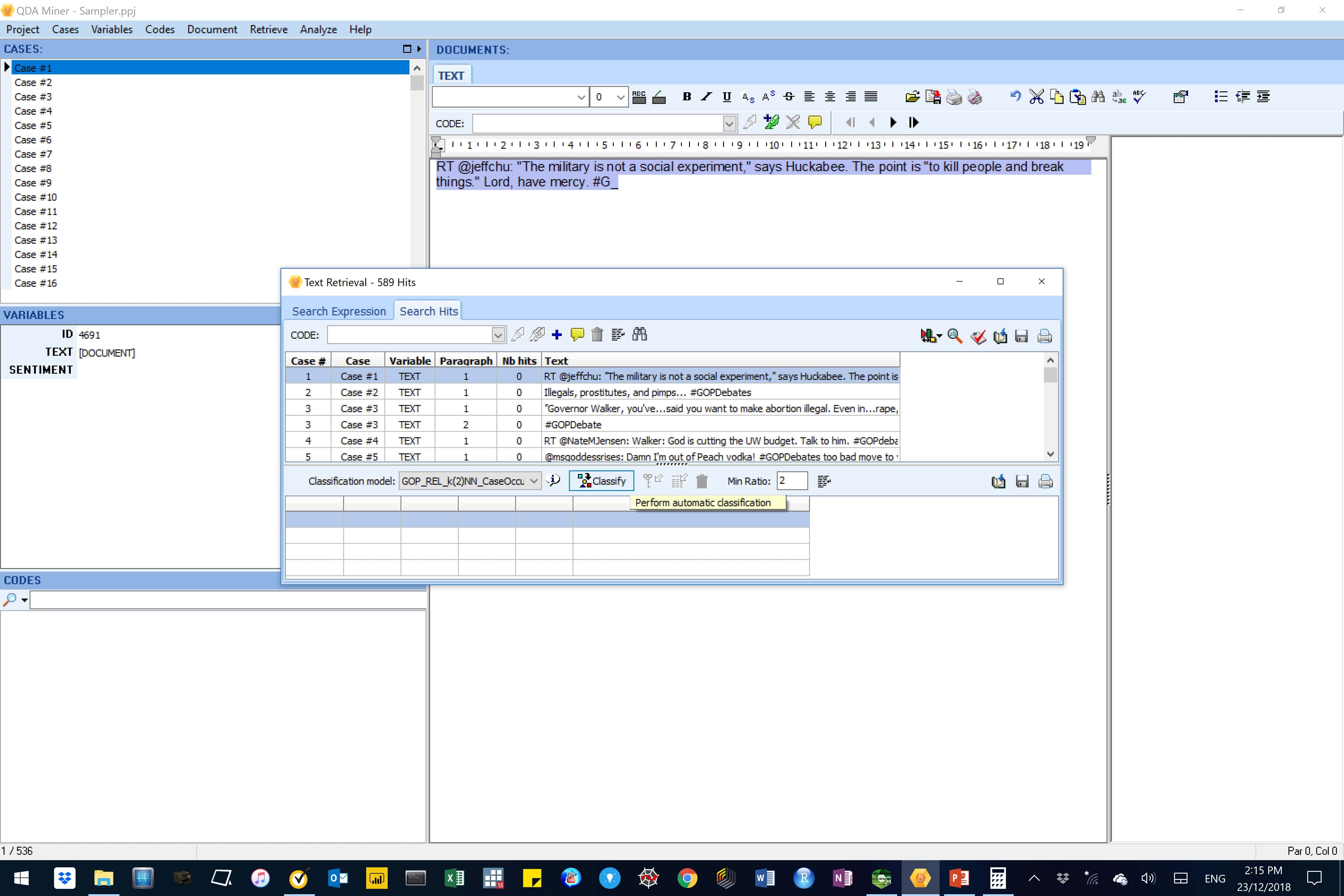
Figure 18: In this image, the sentiment classes in all cases have been predicted.

 

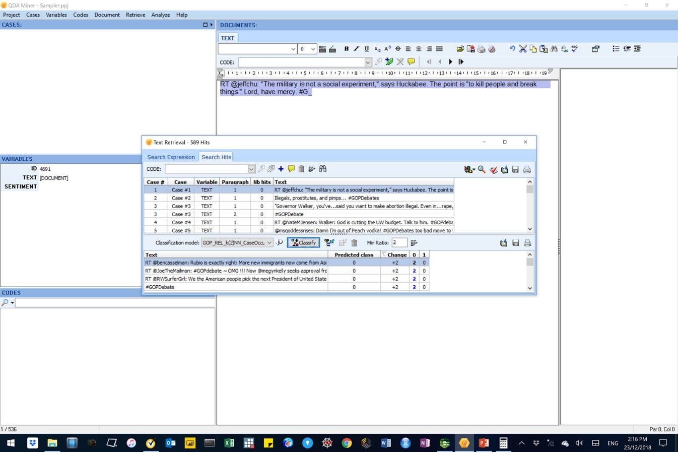
Figure 19: In this image, the sentiment classes in all cases are about to be auto-coded. 

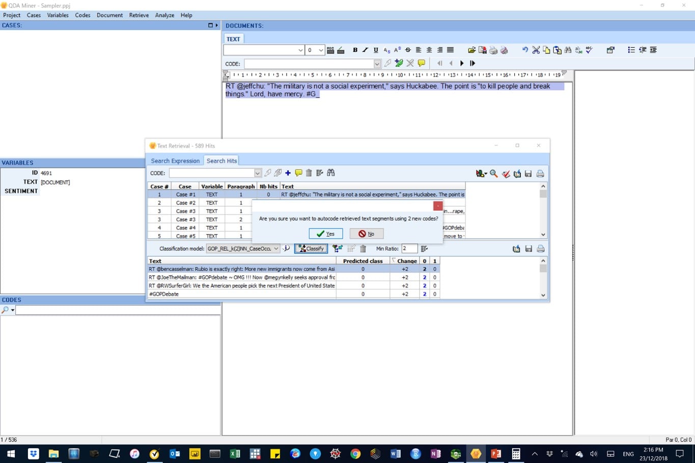
Figure 20: In this image, the sentiment classes in all cases have been auto-coded. Codes 0 and 1 represent the negative and positive sentiments, respectively. 

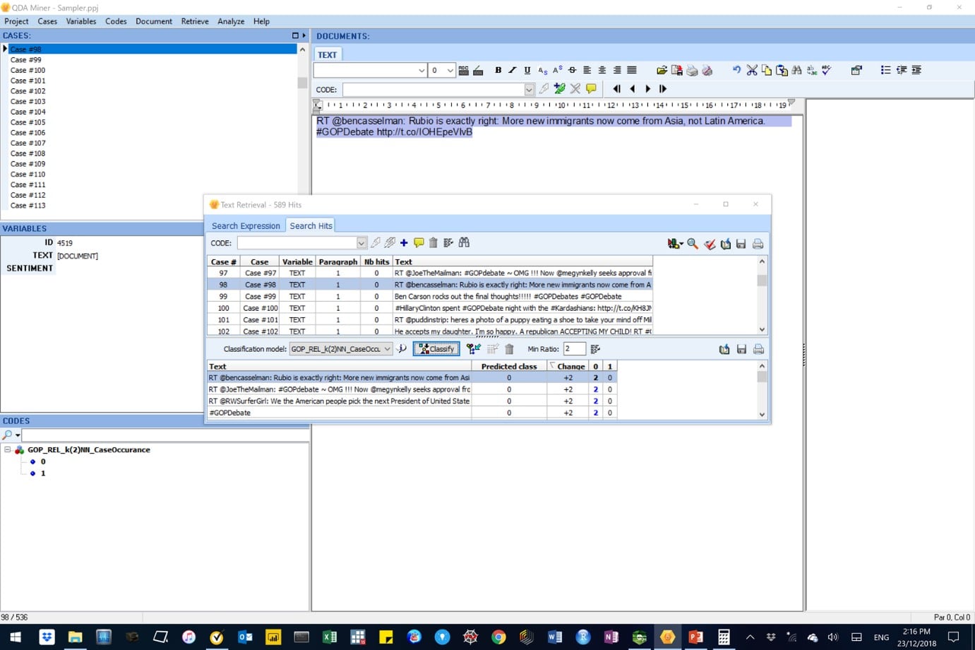
Figure 21: In this image, the text was encoded as 0 to represent a negative sentiment.

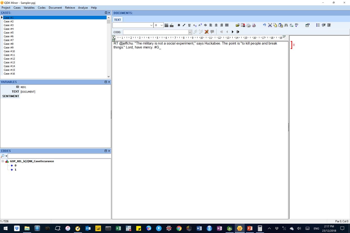
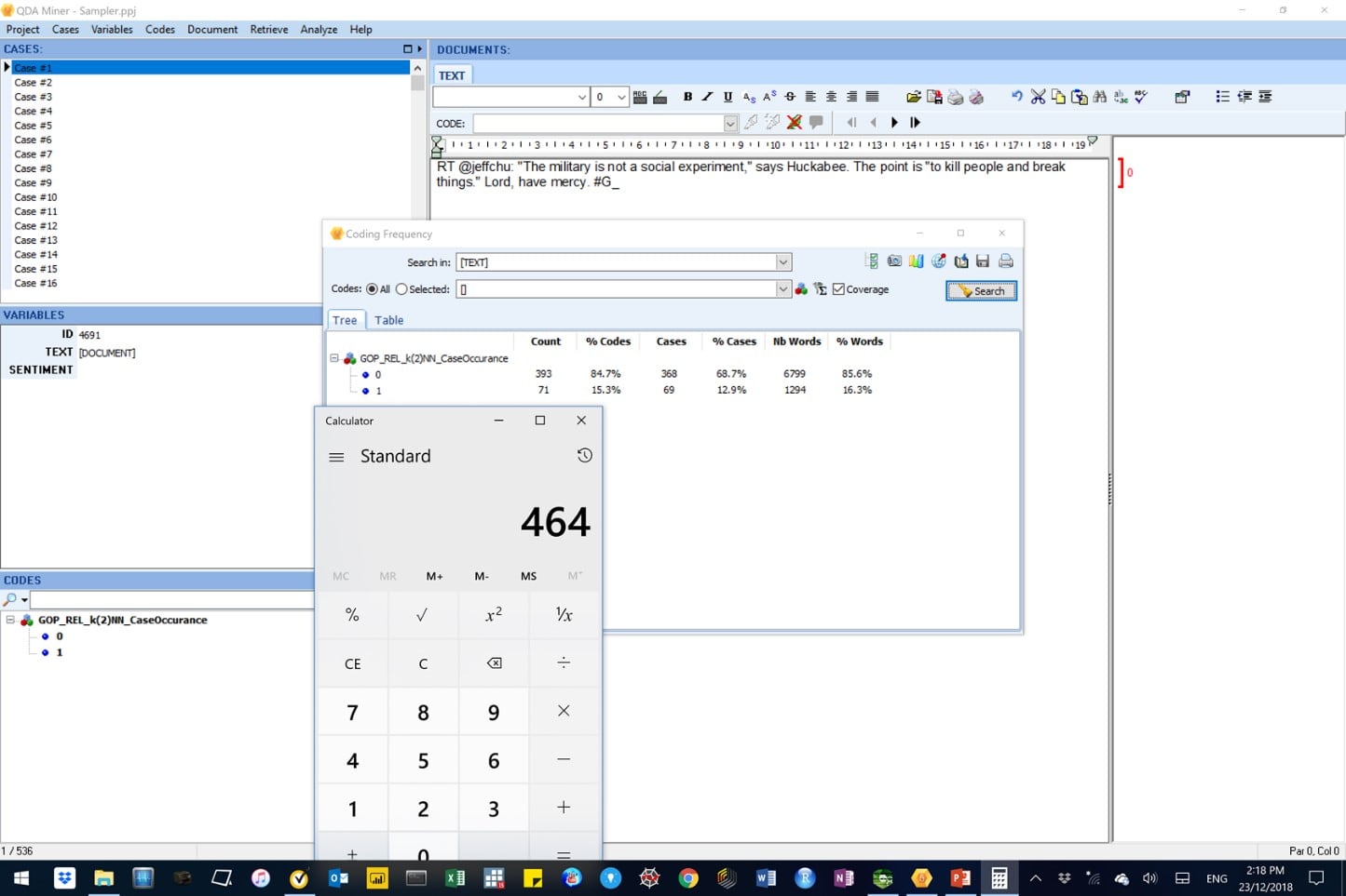
Figure 22: In this image, some summary statistics from the autocoding process are shown under the ‘Tree sub-tab’ of the Coding Frequency tab.

The above results suggest that:

464 out of 536 cases that were successfully encoded. This means the rest (73) was not; andOf the encoded cases, the majority (393 or 84.7%) were predicted as negative sentiments (i.e. code 0) while the rest (71 or 15.3%) were predicted as positive sentiments (i.e. code 1).

Figure 22: In this image, the code retrieval process has picked up 464 cases that had been auto-encoded. We see details of each case, including the sentiment code and case id.

The above results were exported to EXCEL for further analysis. We appended the true sentiment codes that had been stripped-off during document preparation. We then estimated the percentage accuracy.

Table 1: Confusion matrix for the AML-DC model.

predicted

A confusion matrix is a useful tool to assess the performance of an automatic document classifier.

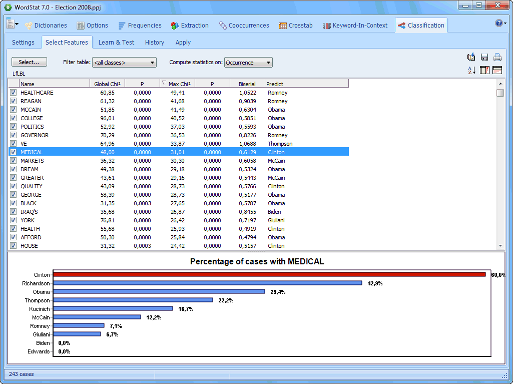The Feature Selection page of the automatic document classification feature allows one to manually or automatically select keywords

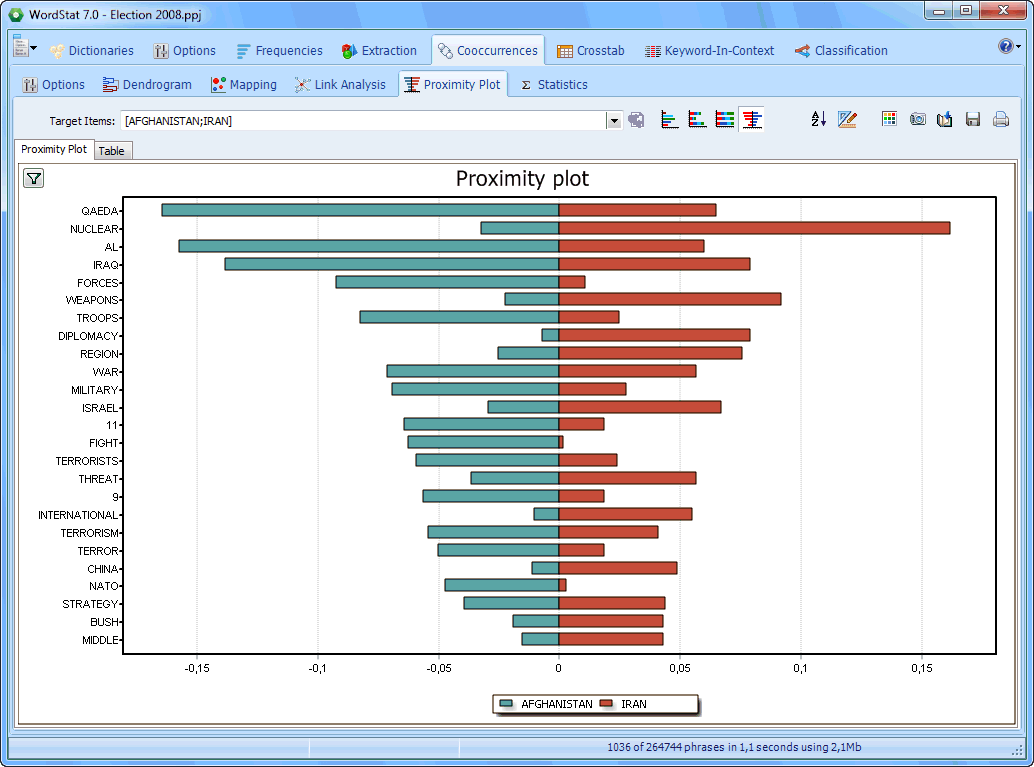Proximity plots may be used to represent the distance from one or several target keywords to all other words

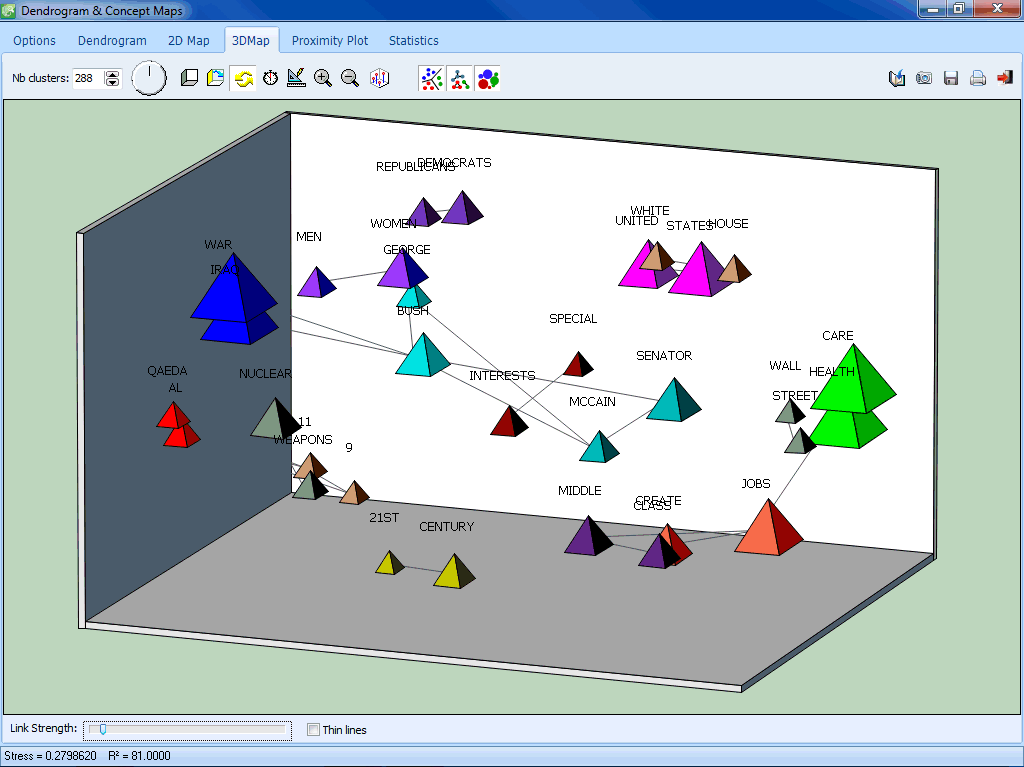This multidimensional scaling displays lines representing the strength of association between data points.

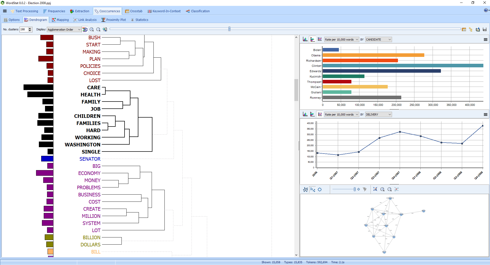Hierarchical clustering is a useful exploratory tool to quickly identify themes or groupings of documents.

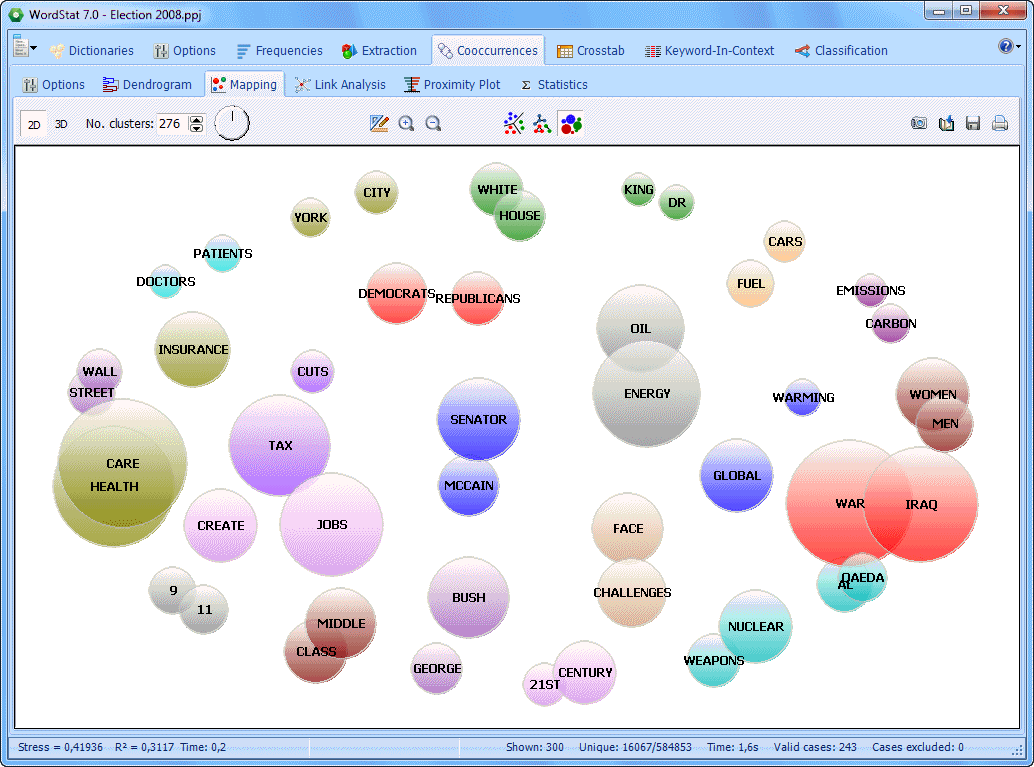Multidimensional scaling maps may be used to represent the co-occurrence of keywords or similarity of documents

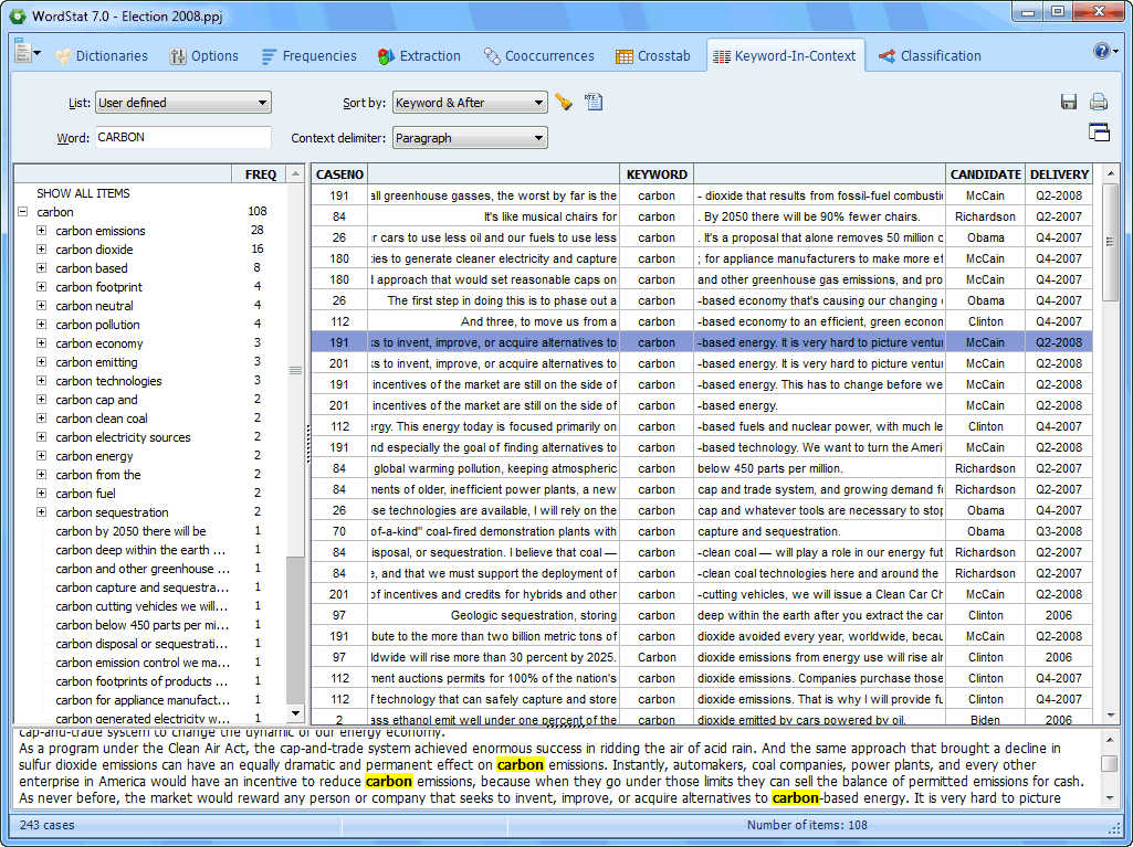The Keyword-In-Context (or KWIC) page allows one to display the context of specific words, word patterns or phrases.

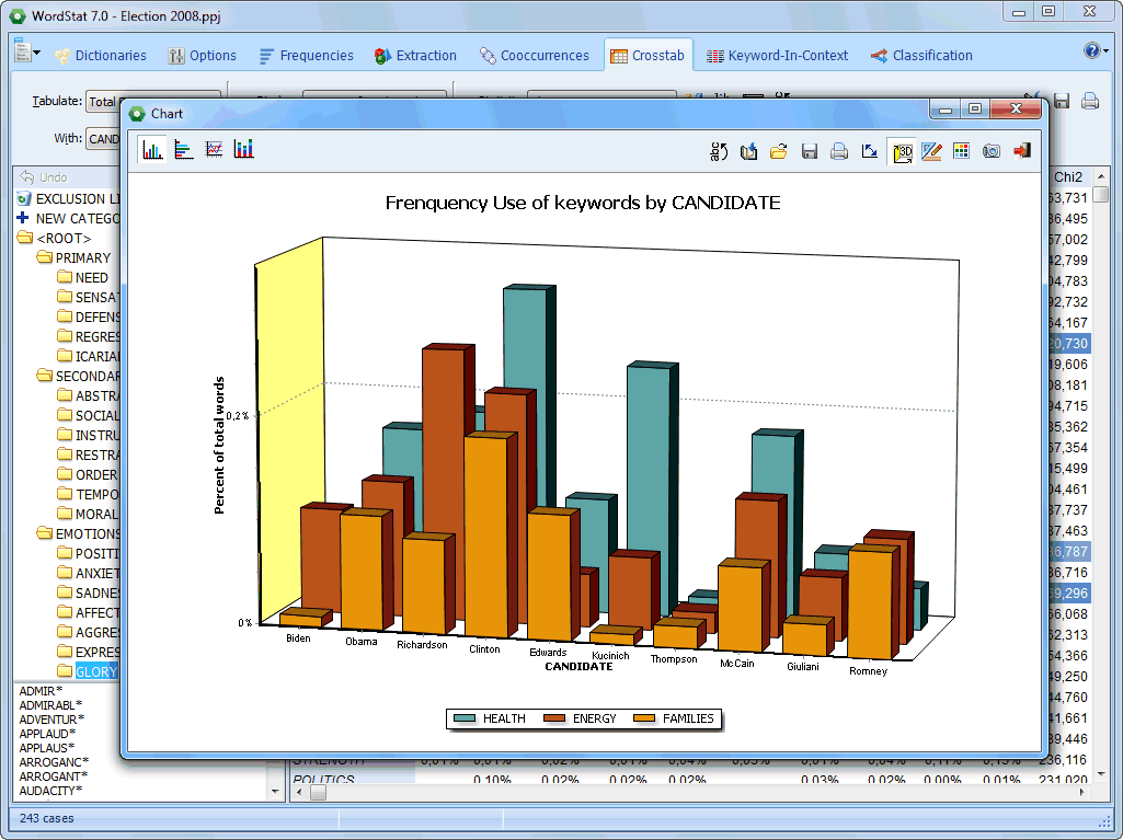Bar charts can be used to represent codes frequencies

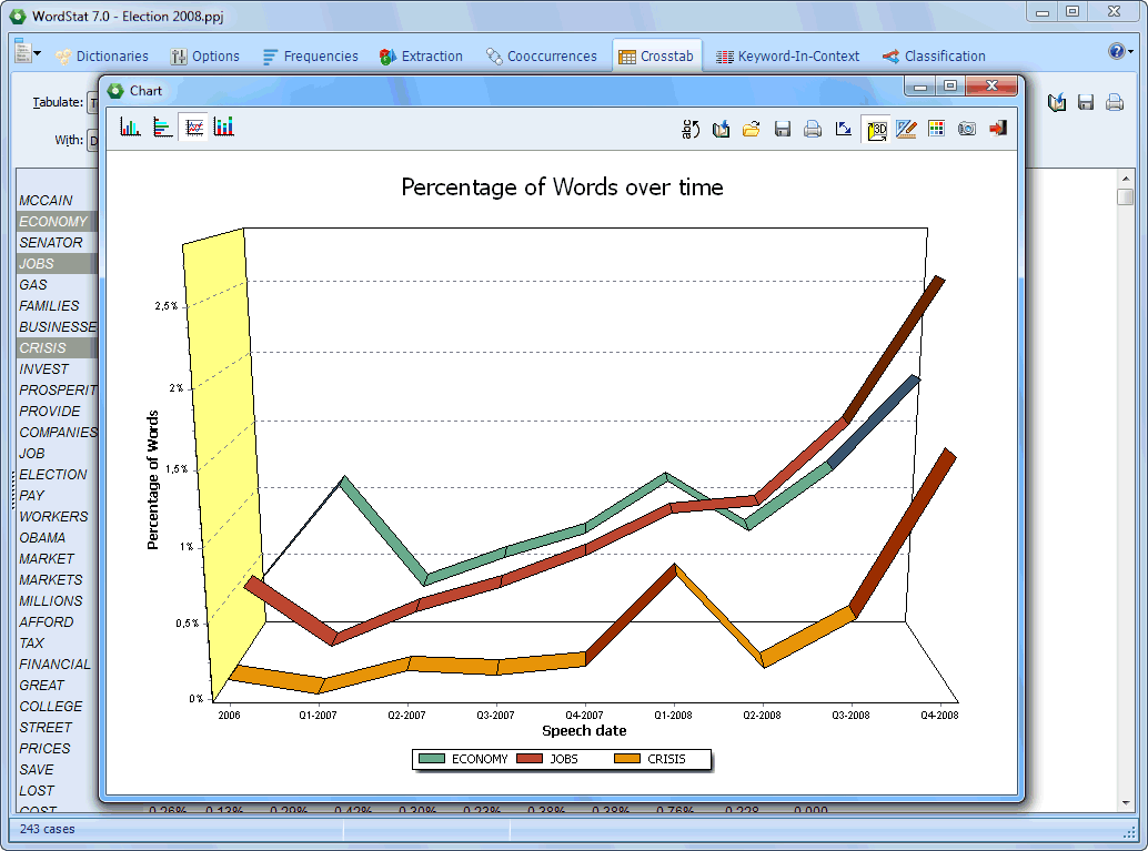Temporal trends of content categories overtime may be plotted using line charts.

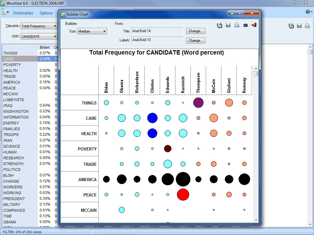Bubble charts are graphic representations of contingency tables where relative frequencies are represented by circles of different diameters.

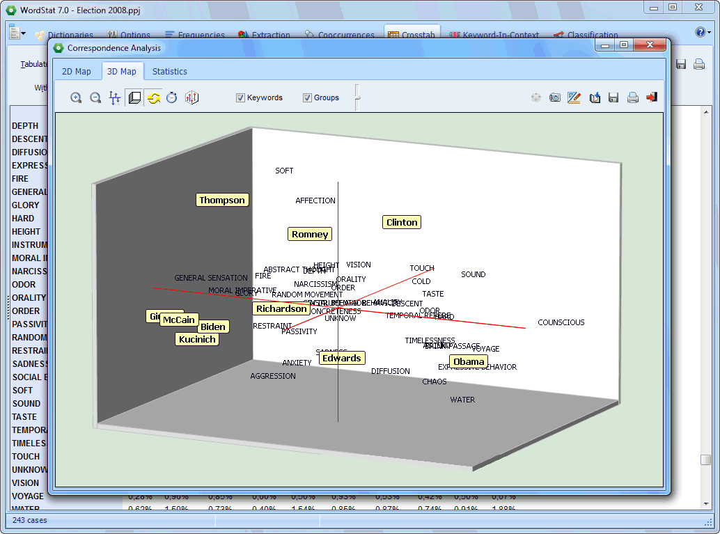Correspondence analysis is a powerful exploratory technique to identify relationships between keywords and categorical or ordinal variables.

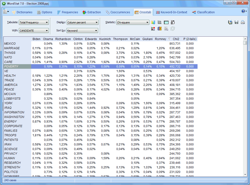The Crosstab page allows one to compare keyword frequencies across values of numerical, categorical or date variables.

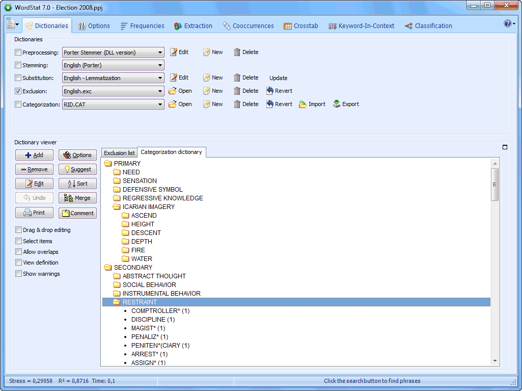The Dictionary page allows one to adjust various text analysis processes, create and modify dictionaries, exclusion and substitution lists.

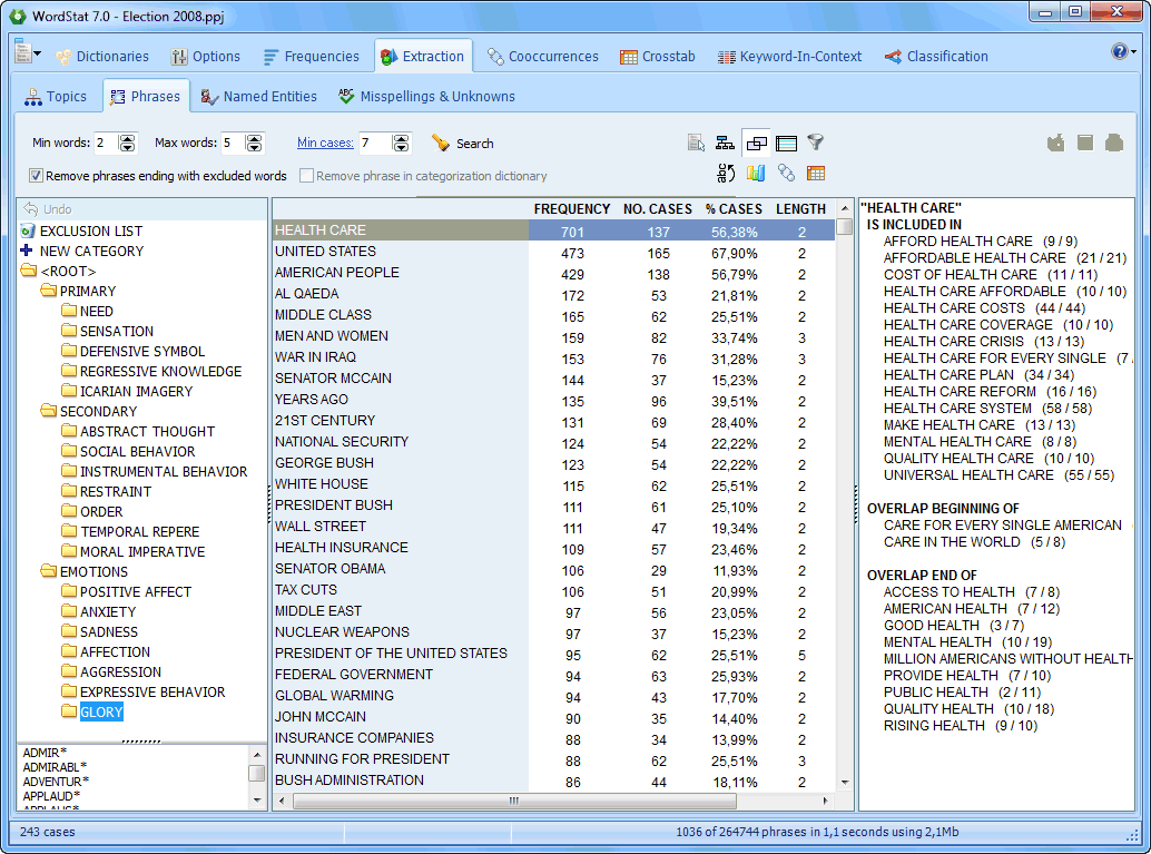The Phrase Finder feature allows one to easily extract the most common phrases and idioms.

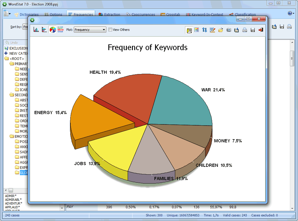Bar chart, pie charts and word clouds can be easily produced.

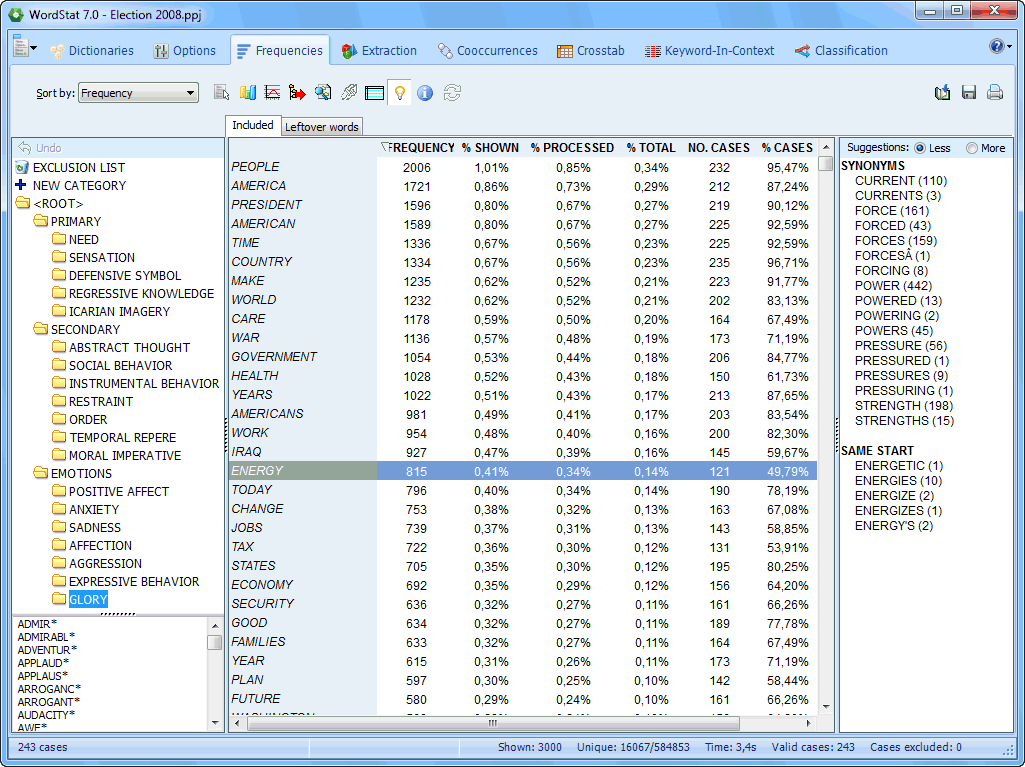The Frequency page displays a frequency table of keywords or content categories. A suggestion panel on the right suggest synonyms and related words.

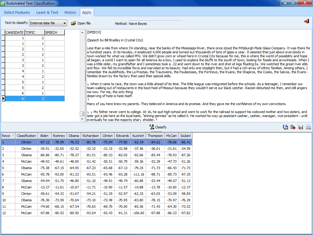The Apply page allows one to categorize a single document, a list of files, or text variables in the current or an external data file.

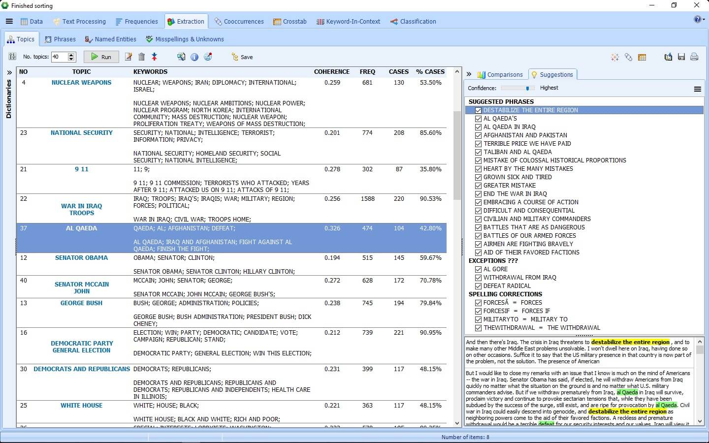Get a quick overview of the most salient topics from large text collections by using state-of-the-art automatic topic extraction techniques.

Table 1 suggests that negative sentiment cases  more accurately (i.e. 354/384 = 92%) than positive sentiment cases (i.e. 41/80 = 51%).  The overall accuracy was 85%. We hypothesised that this probably was due to a case-imbalance between negative and positive sentiment cases in data we had used to build the AML-DC model.

We have presented a remedy for the case-imbalance, below.

Applying the WordStat Sentiment dictionary on our AML-DC model encoded documents 

We opened the AML-DC model encoded, Sample(r) project in WordStat and encoded the cases again, but this time, using the WordStat Sentiment dictionary. We saved the WordStat Sentiment dictionary codes on the Sample(r) project as Word Sentiment dictionary.wmodel.

We used QDA Miner to open the now double-encoded Sample(r) project.

The following series of images show co-occurrence, link and proximity analysis results of the Sample(r) project.

Figure 22: In this image, sentiment codes from our AMCL model, (labelled GOP_REL_k(2)NN_CaseOccurance) and those from the Word Sentiment dictionary.wmodel are shown (bottom left panel).  Also shown are these codes for Case # 1 (top right panel).

Co-occurrence analysis

Figure 23: This image shows the code co-occurrence analysis results for the original input data.

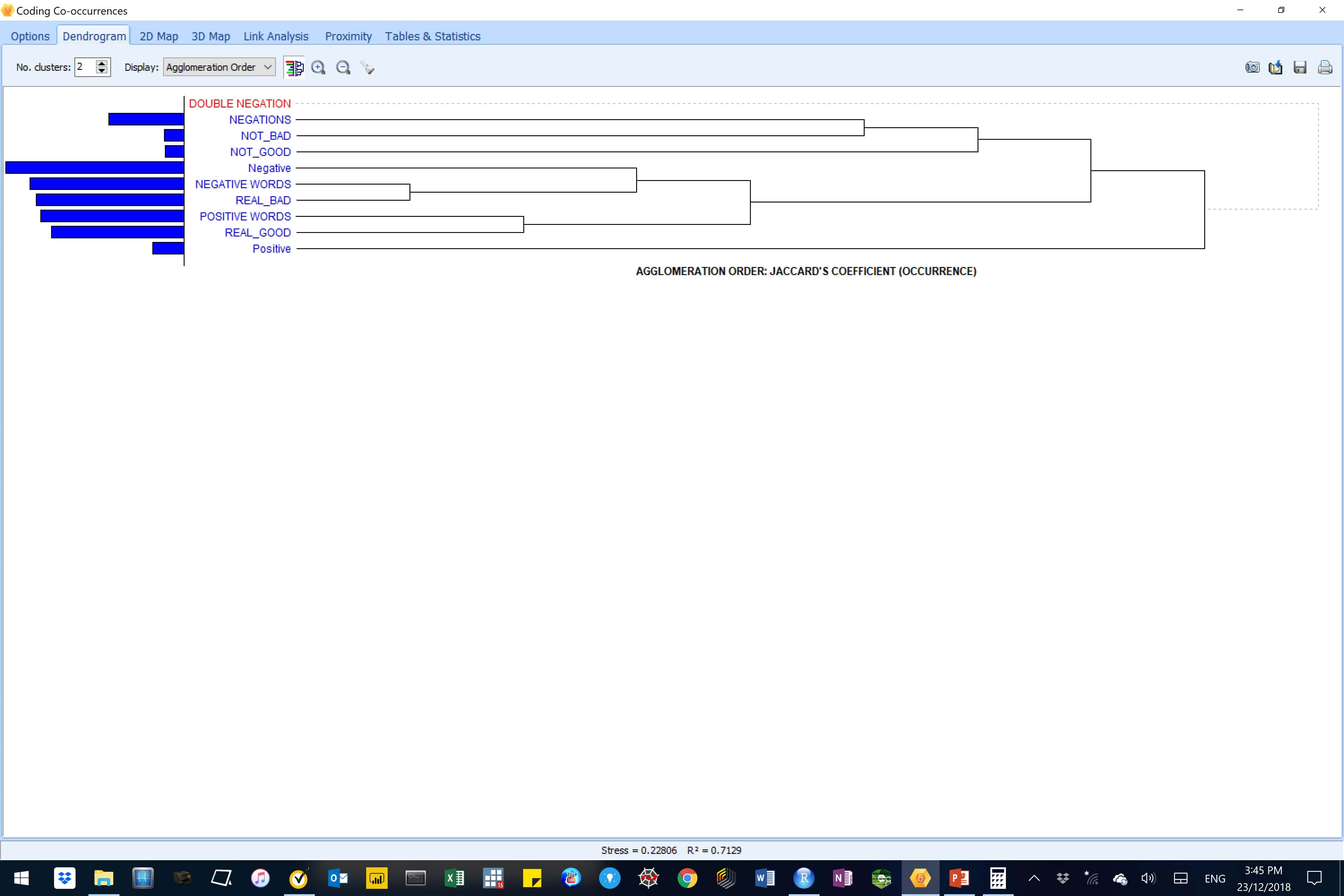
Results suggests that negative codes from the AM-CL model (in lowercase) were more most related to the NEGATIVE_WORDS from the WordStat Sentiment dictionary. Also, positive codes from the AM-CL model (in lowercase) were related to POSITIVE_WORDS and REAL_GOOD words clusters, albeit much less strongly.

Co-occurrences – link analysis

Figure 24: This image shows code co-occurrence analysis results for the original data.

 

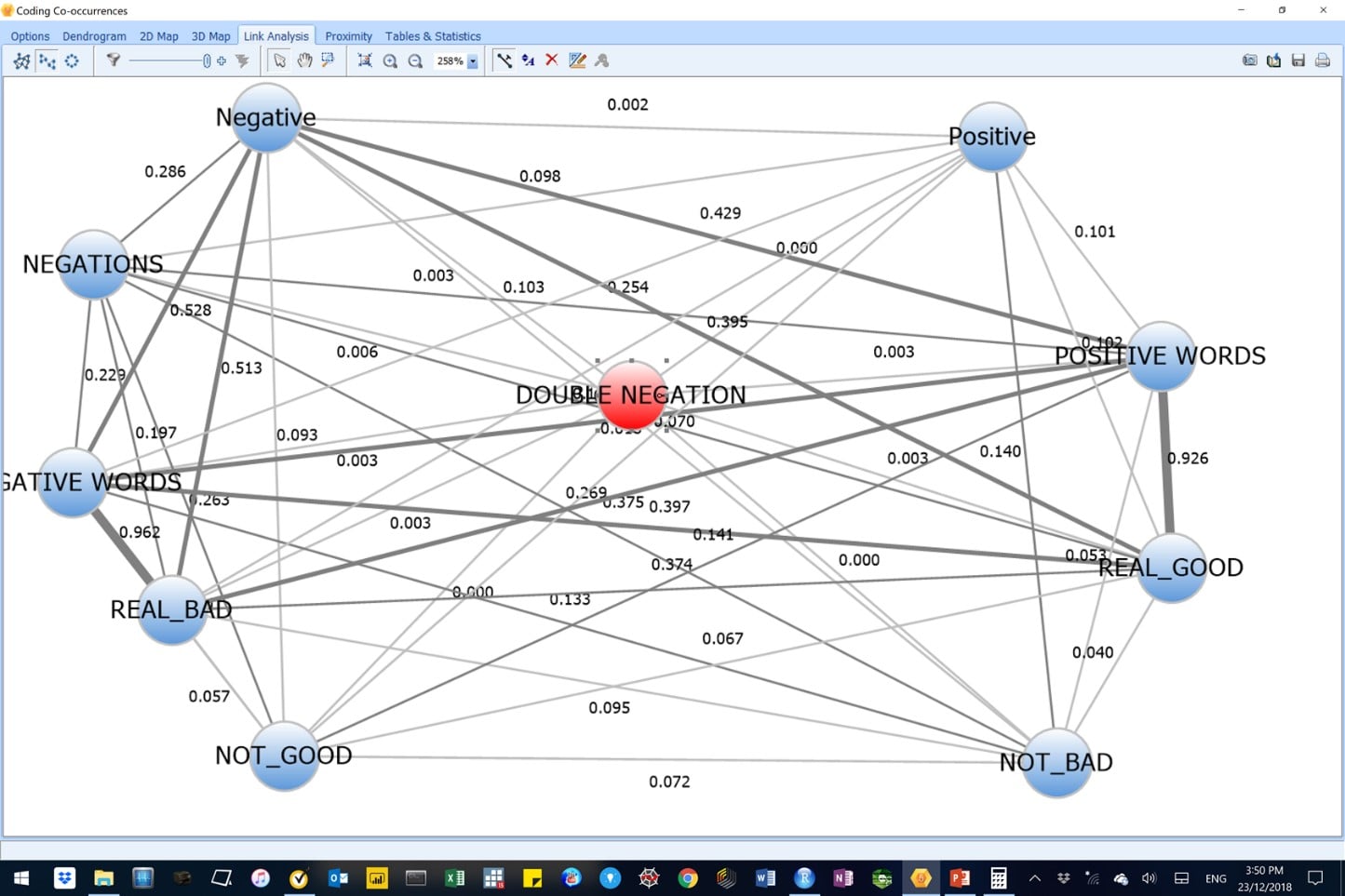
Results concord with the findings from the code co-occurrence analysis, above. Here, we see that relationships between negative sentiment codes from the AM-CL model were stronger (coefficients were higher and lines between the nodes were thicker) than was the case for the positive sentiment codes from the AM-CL model.

Co-occurrences – proximity analysis

Figure 25: This image shows code co-occurrence – proximity analysis results for negative sentiment cases in the original data.

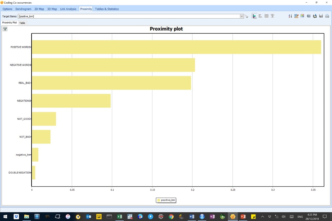
Figure 26: This image shows code co-occurrence – proximity analysis results for positive sentiment cases in the original data.

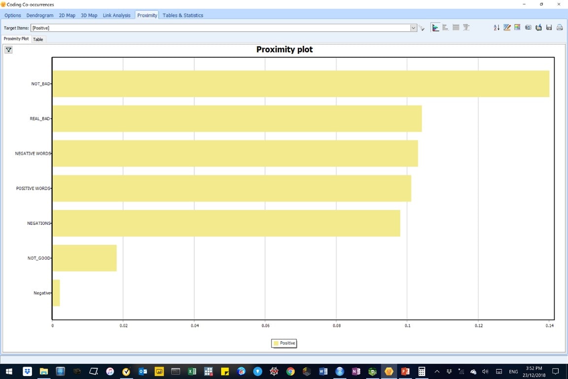
Results also concord with findings from the code co-occurrence analysis.  We also see that REAL_BAD, NEGATIVE_WORDS and POSITIVE_WORDS  from the WordStat dictionary all co-occurred together and but weakly with predicted positive words from the AM-CL model. This is suggests that our model is not as good as it could be.

Correcting code imbalance in the input data prior to model building

As mentioned before, our results suggested that the current AM-CL model was better at predicting negative than positive sentiments. Our model input data had 80% negative sentiment cases and only 20% positive sentiment cases, presenting a case-imbalance in the model input data. This is a common pitfall in machine learning modelling.

To remedy this, we deliberately optimised for positive sentiment cases by keeping all positive cases and choosing only an equal number of negative sentiment cases. We then produced a classification model (see Figure 27) and overlayed the WordStat Sentiment dictionary, as before.

Figure 27:  This image is for a K (2)-Nearest Neighbour AM-CL model built in WordStat, with Inverse Document Frequency (IDF) feature weighting for the balanced dataset. Note the negative (0) and positive (1) sentiment cases are now balanced, roughly 50% each.

We applied the AML-DC model from the balanced input data to unknown corpora, as before. We exported the output to R as a csv file and calculated accuracy in the encoded data, as before.

Table 2, below, suggests that negative sentiment  cases  (i.e. 1,539/1,590 = 97%) and positive sentiment cases (i.e. 1,520/1,578 = 96%) were both very accurately predicted using the AML-DC model built with the balanced input data. The overall accuracy was 97%.

Table 2: Confusion matrix for the AML-DC model using balanced input data.

predicted

Title & description	Date	Host	Language	Registration
Understanding Causes of War, Qualitative Analysis of Diplomatic Archives.	Wednesday, May 08 2024 12h-13h00 EDT	Matthieu Grandpierron Associate professor of international relations and political science, Catholic University of Vendée.	English	Sign up now

The following text and series of images all show the benefit of using the balanced input dataset in model building.

Below is a summary comparison of code-similarity analysis results obtained in QDA Miner from the original and balanced models for positive and negative cases.

Figure 28: Code-similarities between predicted positive cases with the original and balanced input datasets. WordStat Sentiment dictionary codes are capitalised. The negative_knn codes were from the AM-CL models.

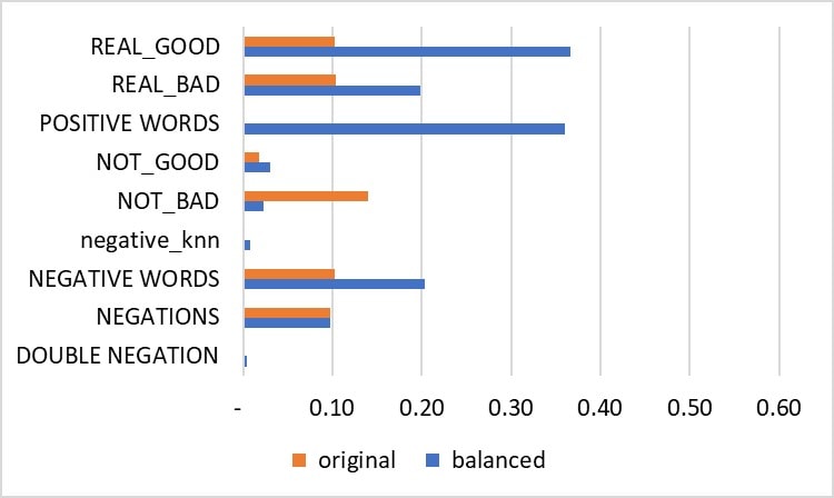
Figure 27: Code-similarities between predicted negative cases with the original and balanced input datasets. WordStat Sentiment dictionary codes are capitalised. The positive_knn codes were from the AM-CL models.

The above results in suggest that correcting for case-imbalance resulted in:

Stronger association of predicted positive sentiment cases in the balanced dataset with the WordStat Sentiment dictionary positive sentiments (i.e. the similarity coefficients for REAL_GOOD and POSITIVE WORDS were higher).Fewer wrong classifications of negative sentiment cases predicted as positive sentiments in the balanced input data (i.e. the similarity coefficients for REAL_GOOD and POSITIVE WORDS were weaker).

Co-occurrences – proximity analysis

Figure 29: This image shows results from a code co-occurrence – proximity analysis of negative sentiments using the balanced input data.

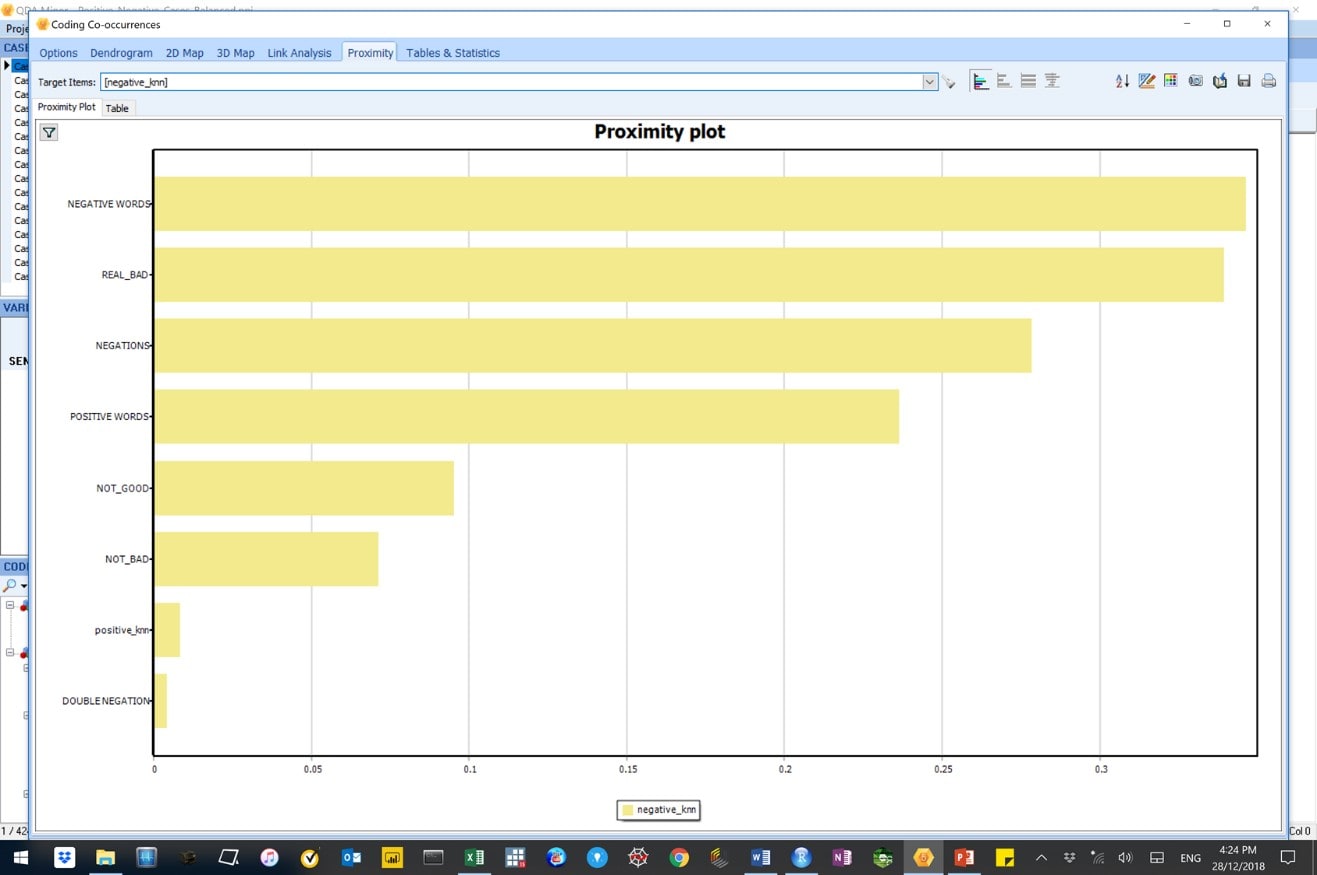
Figure 30: This image shows results from a code co-occurrence – proximity analysis of positive sentiments using the balanced input data.

Results here show an improvement in the ability of the model to correctly predict positive sentiments after correcting for the case-imbalances in the input data.

DISCUSSION

This blog built on the introduction to machine learning key features and processes and factors affecting performance in supervised AML-DC modelling previously outlined by Nyakuengama (2019).

Model performance

In this blog, Naïve Bayes algorithm produced a lower accuracy than the k-Nearest Neighbour (k-NN) algorithm. This is consistent with the literature that suggests that Naïve Bayes models tend to underperform when used with a large number of features (see Nyakuengama, 2019). Our models had between 350 and 670 features.

Also, the literature suggests that Naïve Bayes models perform poorly when features are not independent (see Nyakuengama, 2019).

Benefits of avoiding case imbalances

This study showed that correcting for case-imbalance in the input data, or the unequal instances for different classes, markedly improved the ability of our model to predict the rarer, positive sentiment cases.

Techniques to use prior to- and after-loading corpora into WordStat to improve results

Techniques used in this blogs yielded a good AML-DC model. However, a number of techniques can be employed to further improve the predictive ability of the model. These are include:

Mitigating against case-imbalances by over- and under-sampling, the ROSE package (Lunardon et al., 2014) and the Synthetic Minority Over-Sampling Technique (SMOTE) (Chawla et al., 2000).Experimenting with various WordStat post-processing options:
Pre-processors
WordStat Bag-of-Words options (e.g. n-grams, n-grams  and words, NLTK lemmatization, Porter stemmer and Convert emoticons)
StemmingLemmatization
Experimenting with various WordStat post-processing options:
Adding words with frequency or case occurrence higher or equal to a thresholdRemoving words with frequency or case occurrence higher or equal to a thresholdChanging the threshold of maximum items and their selection criterion (i.e. TF*IDF, frequency and case occurrence).
Cleaning up text during pre-processing:
WordStat default categorization dictionaryDevelop a WordStat exclusion and substitution dictionaries.Adopting third party NLP dictionaries:
Topic specific dictionaries (e.g. for economics, legal and pharmaceuticals)R and Python programming languages
Cleaning up and standardizing the Named Entities during pre-processing:
Use the WordStat Named Entities tabAdopt strategies to manage Named Entities such as those used for Named Entities Recognition (NER) in R and Python programming languages.

CONCLUSION

In this blog provided a practical and detailed walkthrough on the development and application of a AML-DC model to classify unknown sentiment documents.

Then we used the WordStat Sentiment dictionary to measure how well the AML-DC model correctly auto-predicted sentiment in unknown corpora.

Lastly, we demonstrated how correcting for case-imbalances in input datasets is critical, as this markedly improved both the accuracy and predictive ability of the AML-DC model.

BIBLIOGRAPHY

Chawla, N.V., Bowler, K.W., Hall, L.O., Kegelmeyer, W.P. 2000. SMOTE: Synthetic Minority Over-Sampling Technique. Journal of Artificial Intelligence Research, Vol. 16. pp. 321-357.

Figure Eight, 2015.  First GOP debate sentiment analysis – Added: August 11, 2015. http://ptrckprry.com/course/ssd/data/GOP_REL_ONLY.csv

Lunardon, N., Menardi, G. Torelli, N., 2014. ROSE: A Package for Binary Imbalanced Learning. R. Journal, 2014. Vol. 6, (3). pp. 79.

Nyakuengama J.G., 2018a. Stylometry – Authorship Attribution – Early British Fictionists. https://dat-analytics.net/2018/12/02/stylometry-authorship-attribution-early-british-fictionists/

Nyakuengama J.G., 2018b. Prototyping a WordStat/QDA Miner Automatic Document Classification Model For Product Reviews. https://dat-analytics.net/wp-content/uploads/2018/12/Prototyping-A-WordStat-QDA-Miner-Automatic-Document-Classification-Model-For-Product-Review.pdf

Nyakuengama J.G.,  2019.  Part I: Automatic Machine Learning Document Classification – An Introduction. Full reference details to be advised.

QDA Miner/WordStat User’s Manual 2018. https://provalisresearch.com/