本文深入探讨了因果关系、相关性以及混淆因素之间的复杂关系，揭示了在观察数据中，相关性并不一定意味着因果关系，以及如何可能存在因果关系却无法观察到相关性。文章通过图表和实例，解释了因果推断的基本概念，如潜在结果、处理效应和选择效应，并探讨了混淆因素如何导致错误的结论。文章最后强调了随机化的重要性，以及在没有实验数据时，经济学家们如何尝试接近实验理想状态。

💡 **因果关系与潜在结果：**因果关系指的是一个处理（例如服用维生素C）对结果变量（例如感冒恢复时间）的影响。文章引入了潜在结果的概念，即个体在接受或不接受处理时的两种可能结果。因果效应被定义为潜在结果之间的差异，但由于我们无法同时观察到这两种结果，因此产生了因果推断的基本问题。

🤔 **相关性、混淆与选择效应：**相关性指的是在数据中观察到的两个变量之间的关系，而混淆是指由于选择效应的存在，导致处理组和对照组在潜在结果上存在差异。选择效应是指未接受处理组和已接受处理组之间的潜在结果差异。文章通过实例说明了混淆如何导致观察到的相关性与真实的因果效应相反。

🧐 **相关性不等于因果关系，以及因果关系不一定有相关性：**文章通过实例展示了相关性不一定是因果关系的，例如服用维生素E与健康之间的关系，实际上是健康生活方式的人选择了服用维生素E，导致了观察到的相关性，而维生素E本身对健康没有显著影响。文章还阐述了因果关系不一定有相关性的情况，例如在控制系统中，处理被选择性地应用以保持某些东西的恒定，导致观察不到相关性。

✅ **随机化的重要性：**文章强调了随机化的重要性，通过随机分配处理，可以使处理组和对照组在其他因素上保持可比性，从而消除选择效应，更准确地评估处理的因果效应。随机化有助于解决因果推断中的基本问题，即无法同时观察到所有个体的潜在结果，从而更准确地估计因果效应。

Published on June 9, 2025 8:46 PM GMT

I’ve developed a new type of graphic to illustrate causation, correlation, and confounding. It provides an intuitive understanding of why we observe correlation without causation and how it's possible to have causation without correlation. If you read to the end, you'll gain a basic understanding of topics at the frontier of econometrics research. Let's get started!

Causation

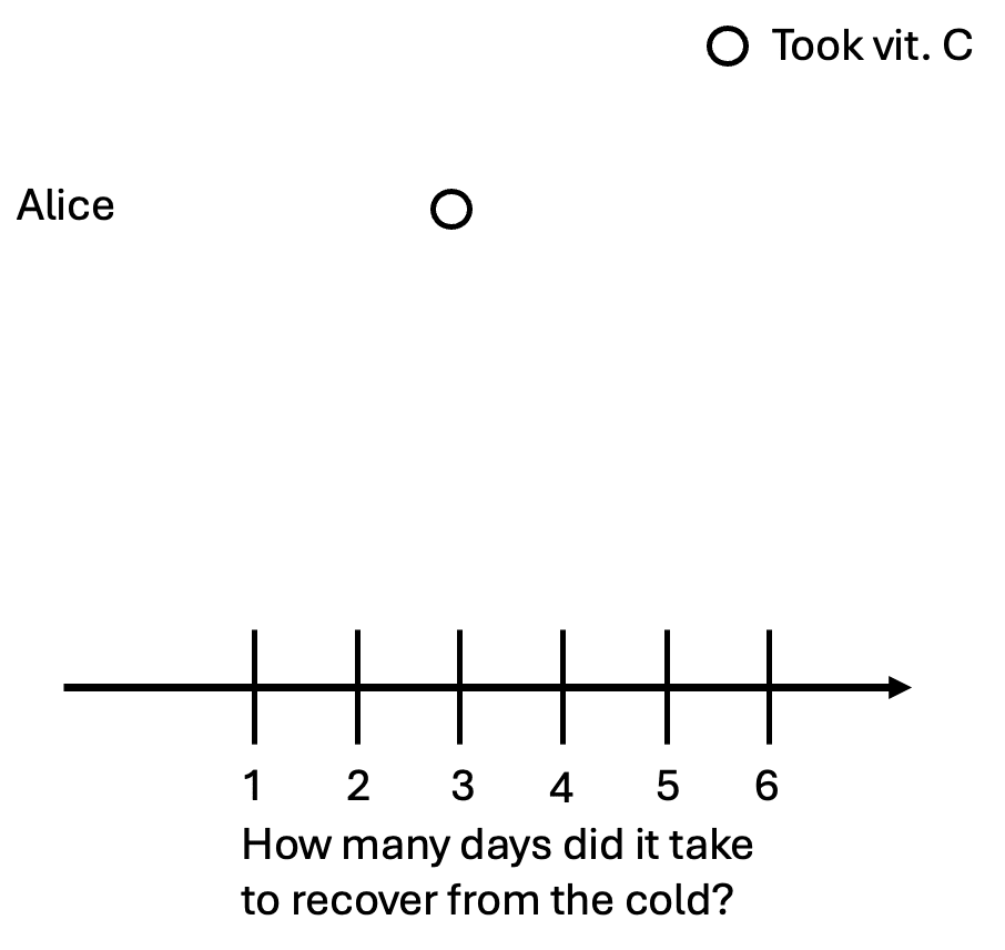
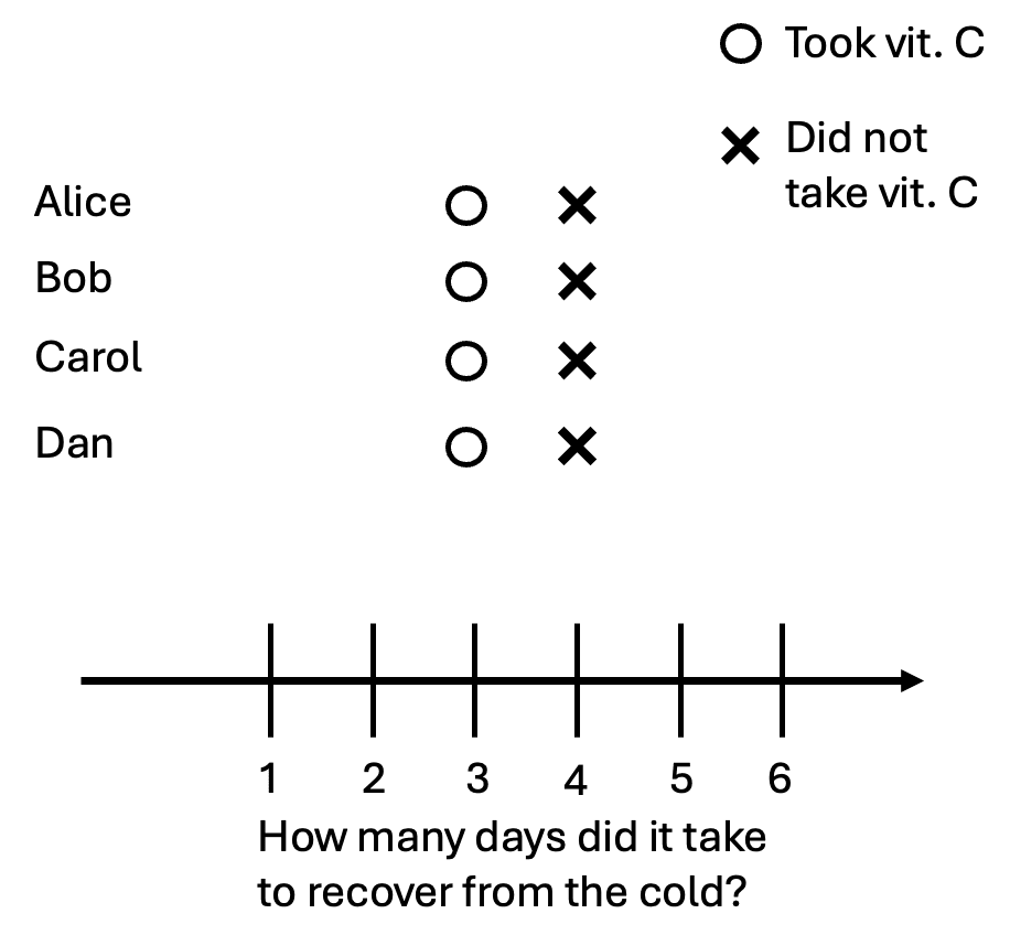
Suppose Alice just caught a cold. She read online that taking vitamin C might reduce the time it takes for her to recover,^[1] so she takes a vitamin C pill and feels better after three days. We’ll denote this as a circle on the graph:

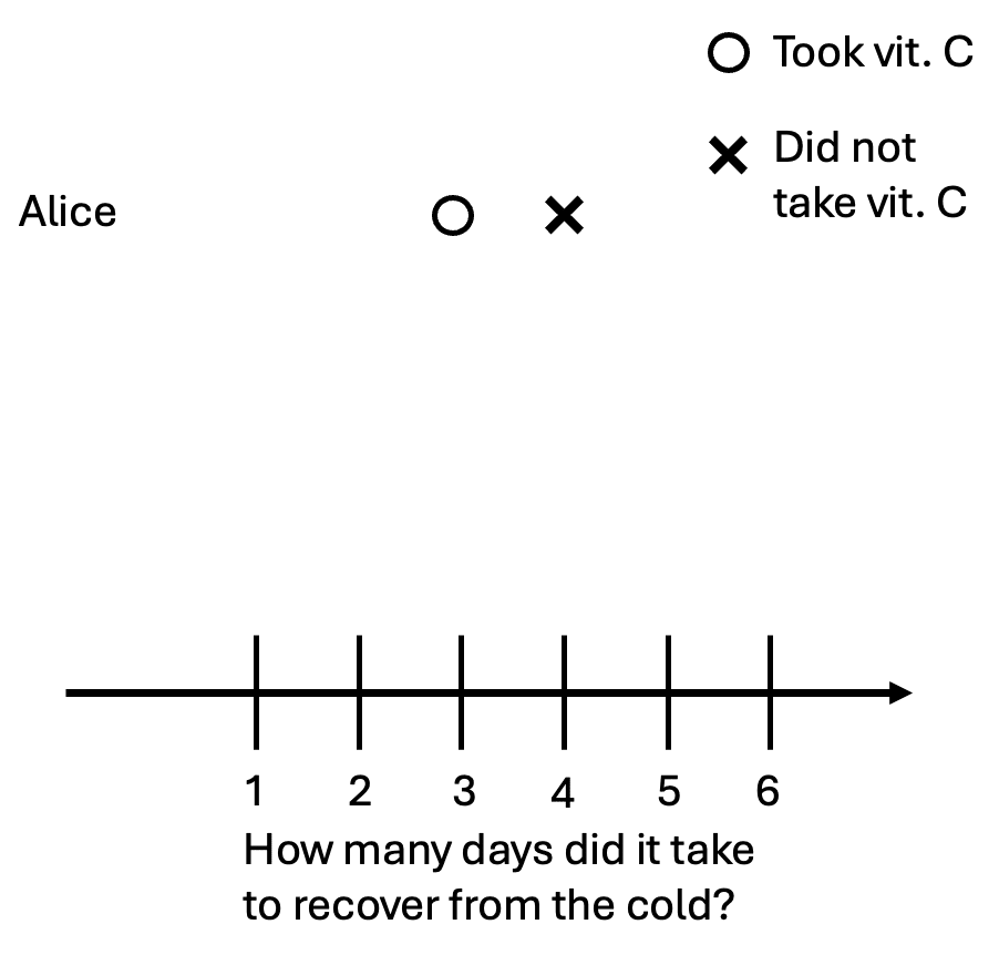
Is this enough to tell if vitamin C helped Alice get better? No. We need to know how long it would’ve taken Alice to recover if she had not taken vitamin C. Suppose that vitamin C works: it would’ve taken Alice four days to recover without the pill. We can denote that as an x on the graph.

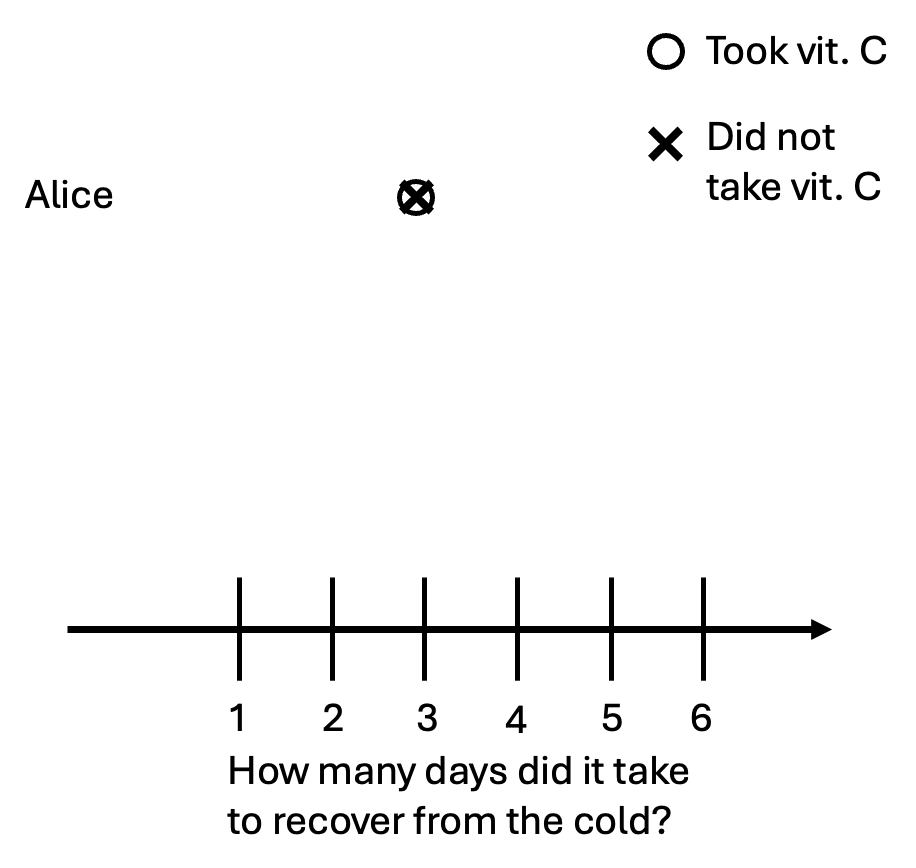
It’s also possible that taking the pill did not help Alice at all. In other words, she would’ve gotten better in three days whether she took a pill or not. We can illustrate this graphically:

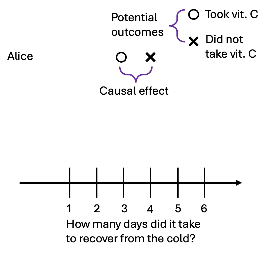
We’ll introduce some terms from the language of causal inference.^[2] The person with the cold (Alice) is our unit of observation. The number of days it takes her to recover is our outcome variable—the thing we want to affect. The vitamin C pill is our treatment, an action a unit can take. The symbols o and x represent potential outcomes. In our example, the potential outcomes are the two possibilities: the number of days it takes to recover with the vitamin C pill, and the number of days it takes to recover without it.

Armed with these new words, we can now define causality:

Causality: The causal effect (or treatment effect) of a treatment is the difference between the potential outcomes.

However, for any given person, we can never observe both potential outcomes. Alice either takes the pill or she doesn’t. This means we cannot directly calculate the causal effect for her. This unobservability is called the fundamental problem of causal inference.

Correlation

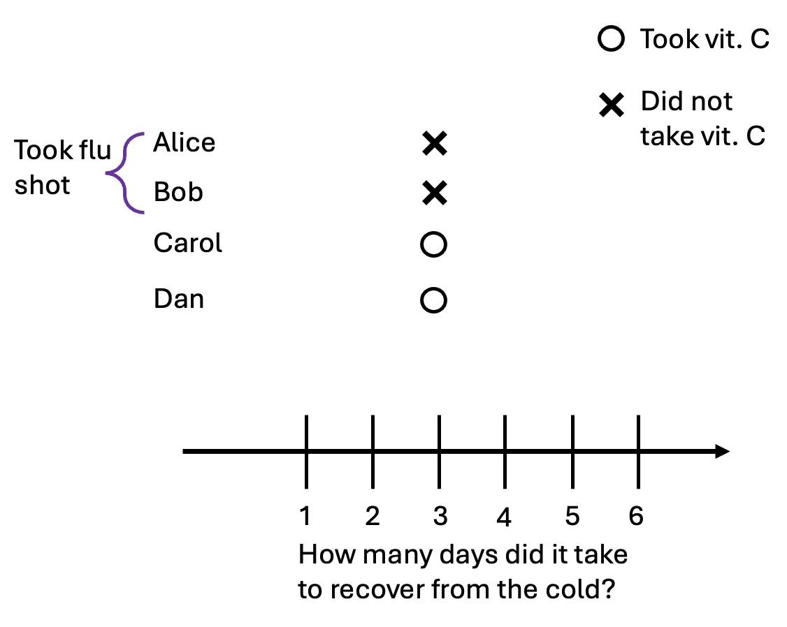
Let’s now consider four people who all got the cold: Alice, Bob, Carol, and Dan. In this scenario, they are all identical: they will recover in three days if they take vitamin C, and recover in four days if they don’t:

Suppose Alice and Bob took the pill, but Carol and Dan didn’t. Here are the data points we can actually observe:

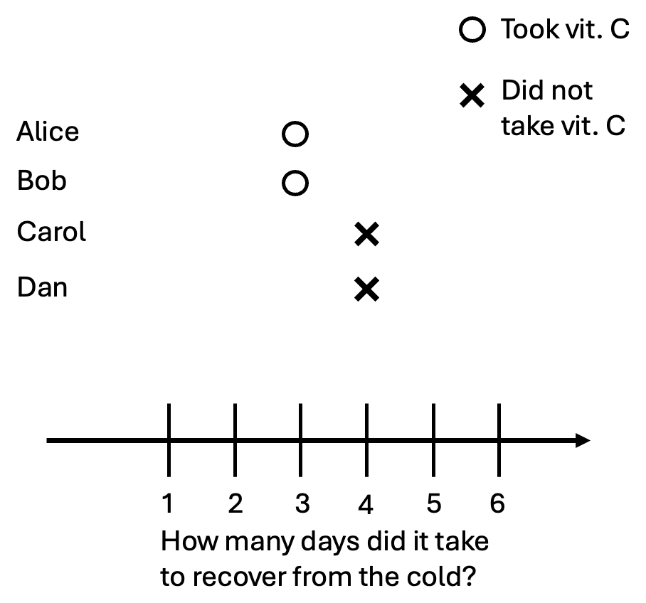
We observe that the people who took the pill got better after three days, and those who didn’t got better after four days. This means that the pill is correlated with people getting better sooner.

Correlation: Correlation is calculated using the observed relationship between two variables in the data. 

Notice the key distinction between correlation and causation: correlation is something we can observe, while causation is focused on the difference between potential outcomes that are never fully observed. However, everyone has identical potential outcomes in this scenario, and the only difference is that Alice and Bob took the pill while Carol and Dan didn’t. In this case, the observed correlation is exactly the causal relationship. 

Confounding

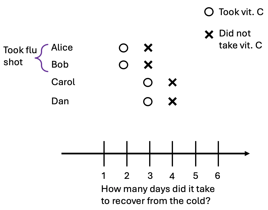
In our previous example, everyone had identical potential outcomes, and the true causal effect was the same as the observed differences. Now, suppose there are two types of people, those who took the flu shot, and those who didn’t. The flu shot reduces the length of someone’s cold by two days, regardless of whether they take a vitamin C pill. In our example, Alice and Bob took the shots, and here are the new potential outcomes:

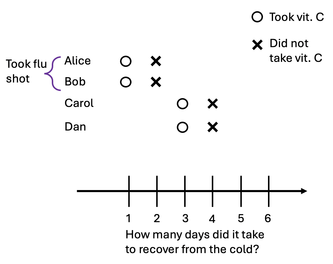
Now suppose that Alice and Bob, feeling invincible from their shot, decided to not bother taking vitamin C after they got the cold. Carol and Dan, regretting the laziness of their earlier selves, take a pill after getting the cold. This is the data we observe:

According to the observed data, those who had vitamin C actually took one day longer to recover from the cold! The correlation between taking the pill actually has the opposite sign as the causal effect. Let’s take a look at the previous graphic again, but this time with the unobserved potential outcomes in grey:

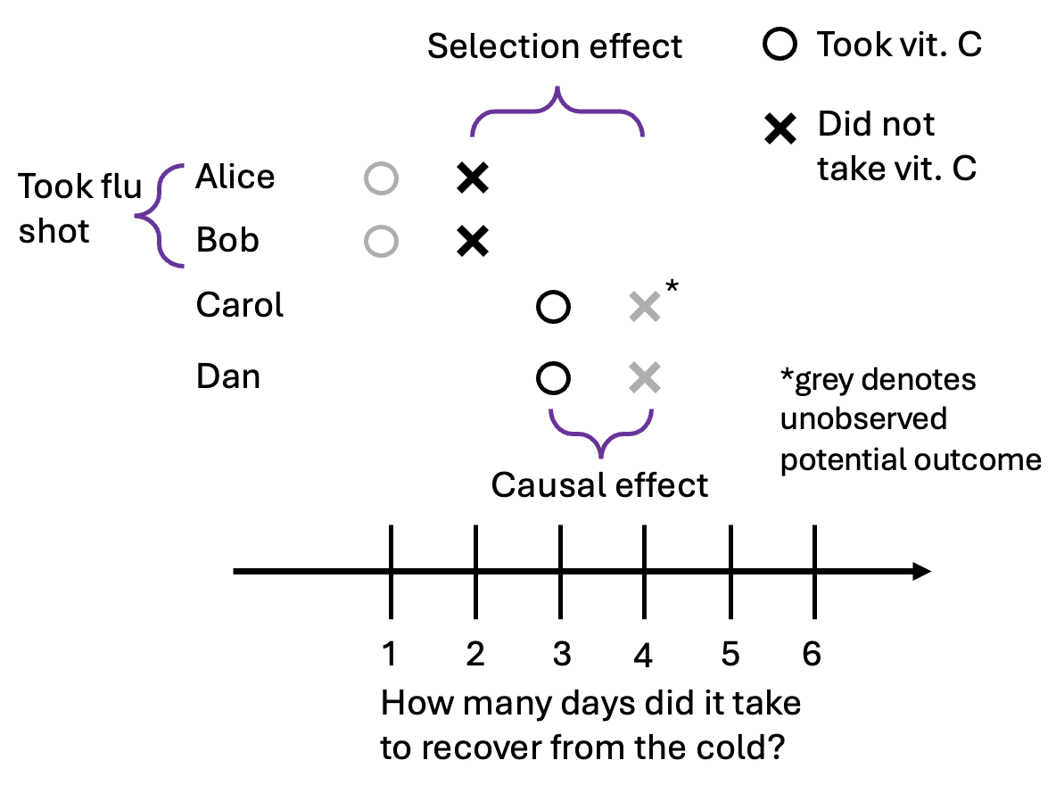
This happened because the people who took the pill (Carol and Dan) had different potential outcomes than the people who didn’t (Alice and Bob). The selection effect is the difference in baseline health between the groups. More formally, it’s the difference in recovery time without vitamin C between those who chose to take the pill and those who did not.

To put it another way:

The causal effect is the difference in potential outcomes within a single unit (e.g., Alice with the pill vs. Alice without).The selection effect is the difference in potential outcomes between treated and untreated units (e.g., Carol's baseline vs. Alice's baseline).

Confounding: Confounding happens when there is a selection effect. That is, the potential outcomes of treated units are different from the potential outcomes of untreated units. In our specific example, taking the pill is confounded with whether someone took the flu shot.

Now I’ll show a few more examples of how the causal effect could be different from the correlation we observe. 

Correlation without causation

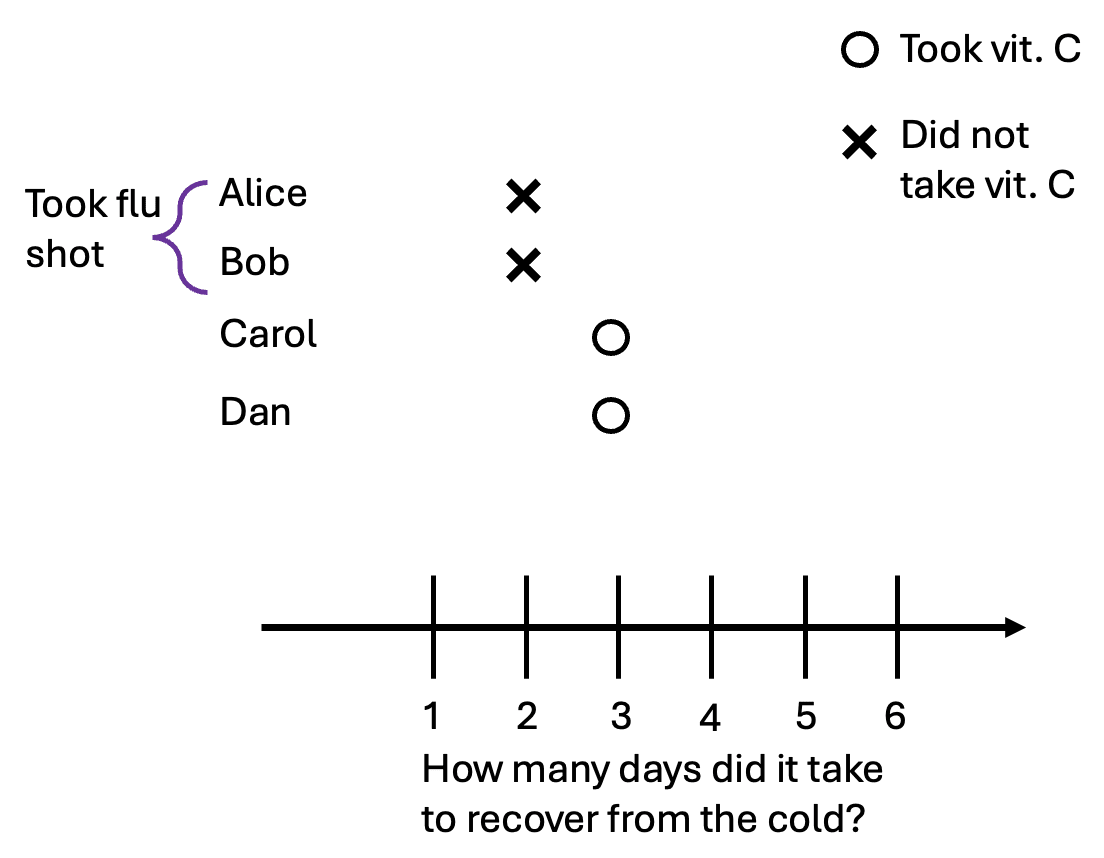
We’ll start by showing an example of correlation without causation. Suppose that vitamin C pills have no effect on how long someone’s cold lasts. o and x are in the same place. We’ll still have Alice and Bob take the flu shot. Here are all of the potential outcomes:

In this scenario, we’ll suppose that Alice and Bob are very health-conscious individuals. They always make sure that they are up to date on vaccines and pay close attention to their health. So here, Alice and Bob take vitamin C, while Carol and Dan do not. (This is the opposite of the selection that occurred in the previous example). We observe the following data:

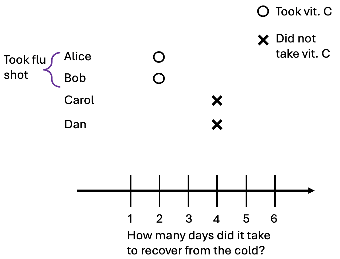
Because of confounding, those who took vitamin C took two fewer days to recover from the cold, even though vitamin C had no causal effect on how long it took for them to recover. 

We have empirical evidence that stories like this—where health-conscious individuals select into treatments with zero causal effects—play out in real life. In the early 1990s, there were some studies showing that vitamin E supplements are good for you. This led to a large increase in vitamin E sales until 2005 when updated studies from randomized trials showed that vitamin E actually has no (or even a negative) effect on health. 

Oster (2020) found that between 1990 and 2005, people who took vitamin E had 25% lower mortality, while after 2005 vitamin E users only had 10% lower mortality. People who took vitamin E supplements were also, for example, much less likely to smoke. This suggests that many people who already had healthy lifestyles started taking vitamin E (which had little causal effect on their health), leading to a large observed correlation between vitamin E use and health outcomes. 

Importantly, the correlation between vitamin E and health remains statistically significant even after we control for various observable outcomes, such as education, income, smoking habits, exercise, vegetable consumption, and more. This suggests that there are unobservable differences between those who took vitamin E and those who didn’t which led to the observed statistical relationship.^[3] 

Causation without correlation

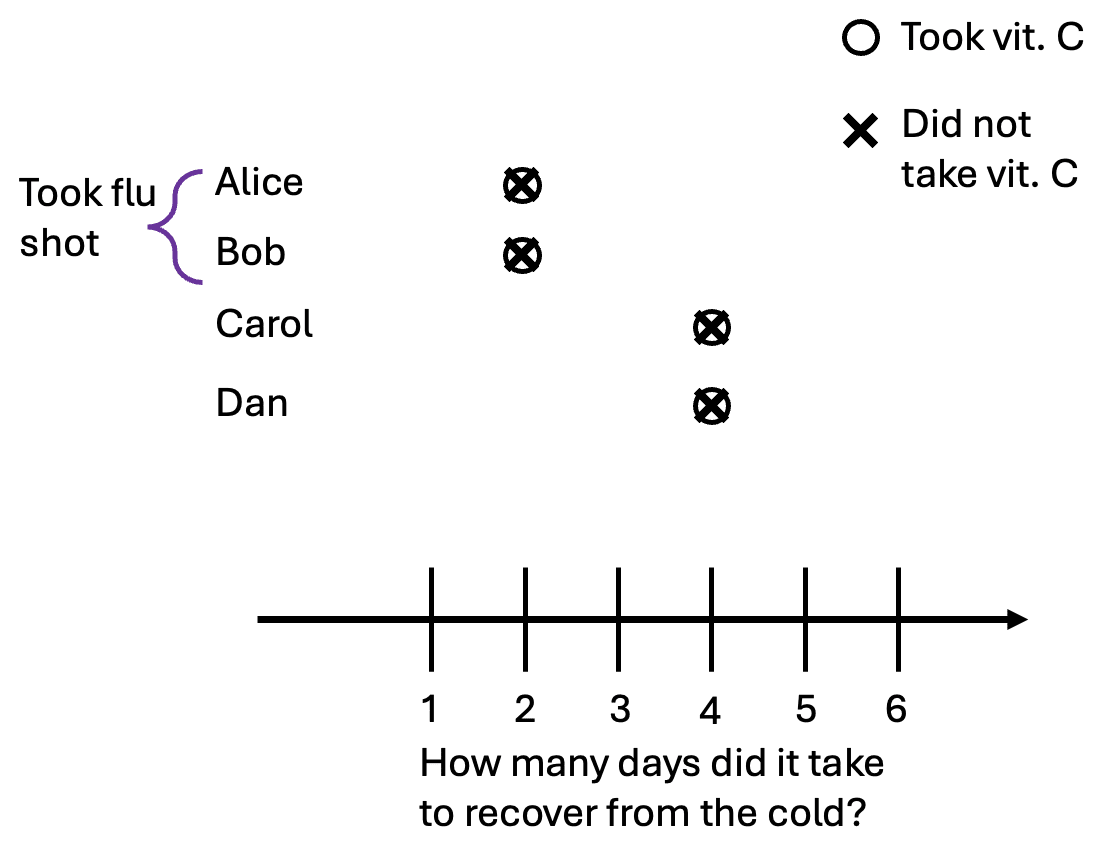
“Correlation does not equal causation” is something people often say. But does causation imply that things have to be correlated? No. We can demonstrate this with a simple modification to our first example in the confounding section. Now, taking the flu shots only reduces the time it takes to recover by one day. Here are our potential outcomes:

Following the first example, Alice and Bob do not take the vitamin C pill while Carol and Dan do. We observe that everyone took three days to recover from the cold, regardless of whether they took a pill or not. In this case, the selection effect and causal effect cancel each other out exactly:

This example may seem unnatural, but causation without correlation is common in control systems where the treatment is selectively applied to keep something constant. For example, consider how much power an air conditioner uses and the temperature inside a climate-controlled room. Turning the AC power up decreases the temperature, which is naturally cooler at night.

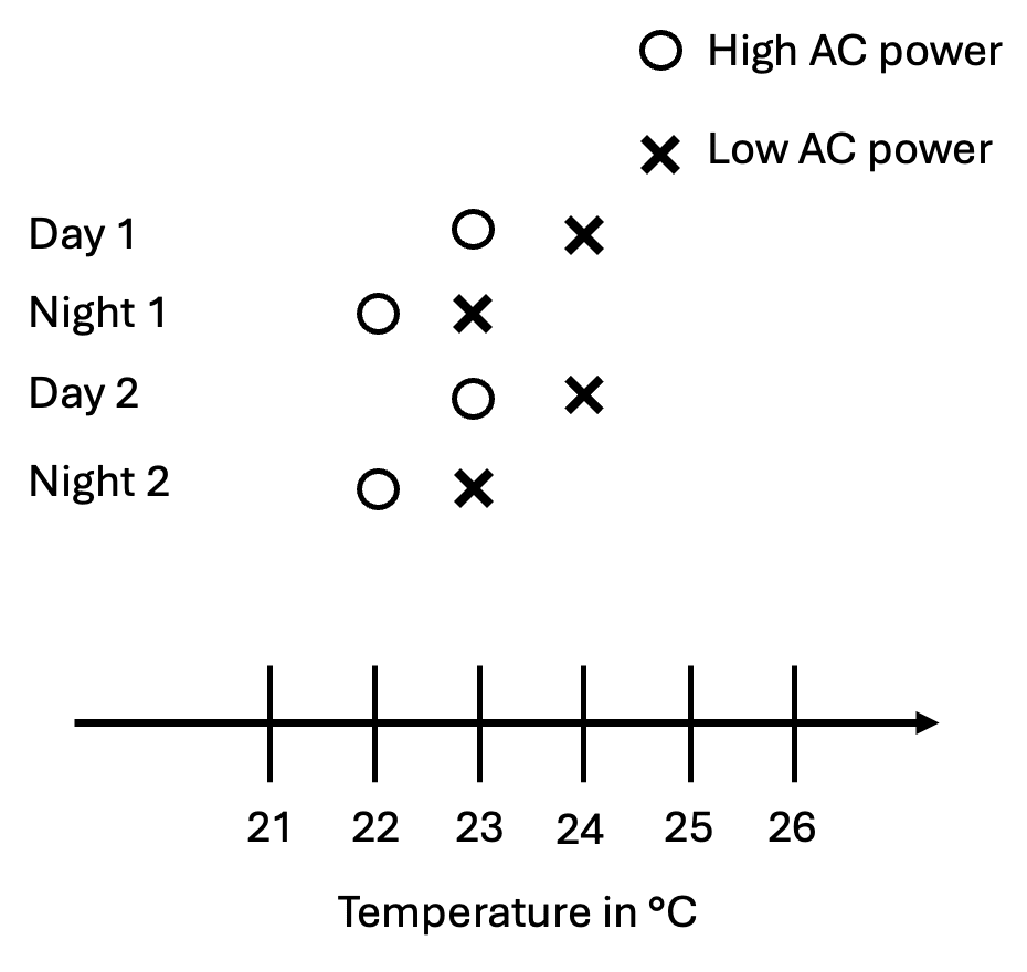
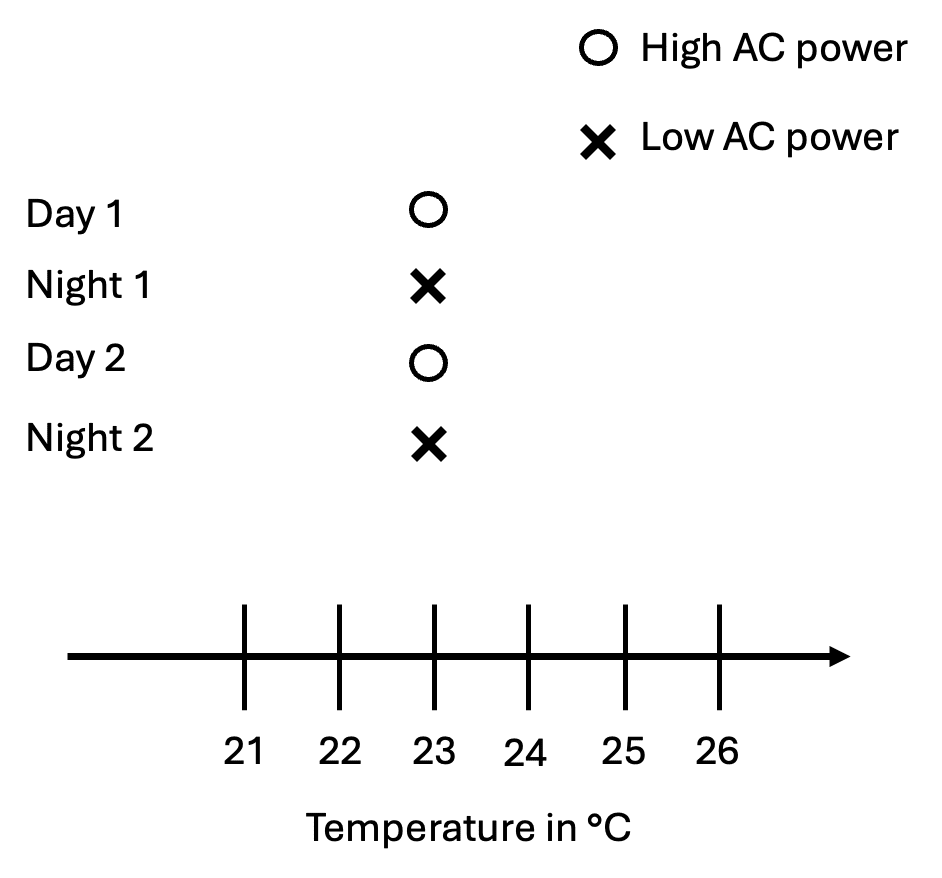
If we set the AC to 23°C, it’ll alternate between high and low power, and we’ll observe zero correlation between AC power and the temperature in a room, even though higher power causes the temperature in a room to drop. 

Why we randomize

The fundamental problem in causal inference is that we can never observe more than one potential outcome for every unit, yet the value we’re trying to find–the causal effect–is defined in terms of the difference in potential outcomes. If we randomize who receives the vitamin C pill in a large sample, then the people who got the flu shot and those who didn't will be distributed roughly evenly across the "treatment" and "control" groups. As a result, the two groups become comparable.

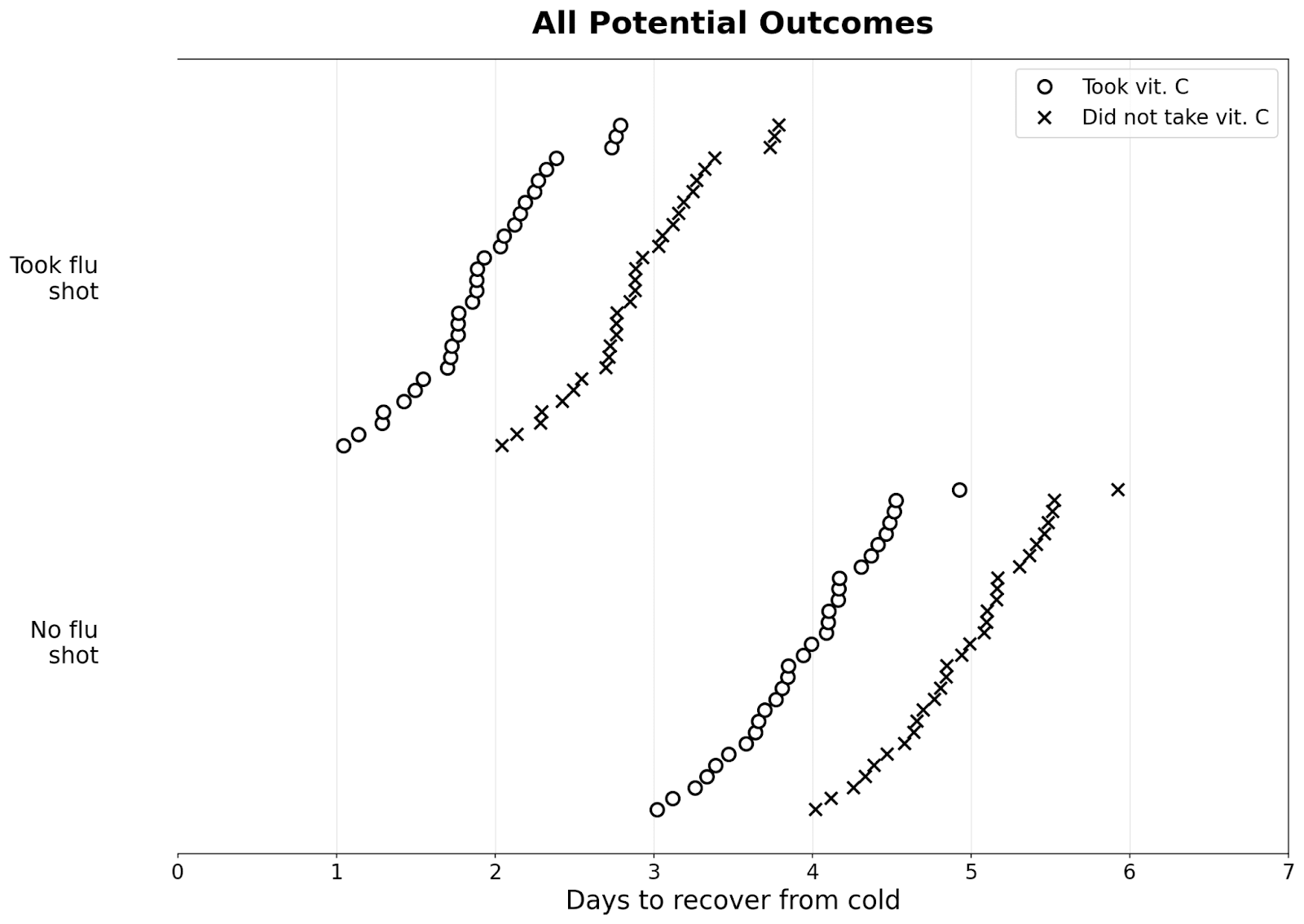
Suppose we have many people who got a cold; some took a flu shot, and some didn’t. Below are their potential outcomes: (I’ve added some noise so they all take slightly different amounts of time to recover)

If we randomize, then about the same number of people get the pill in both groups, as seen in the graph below:

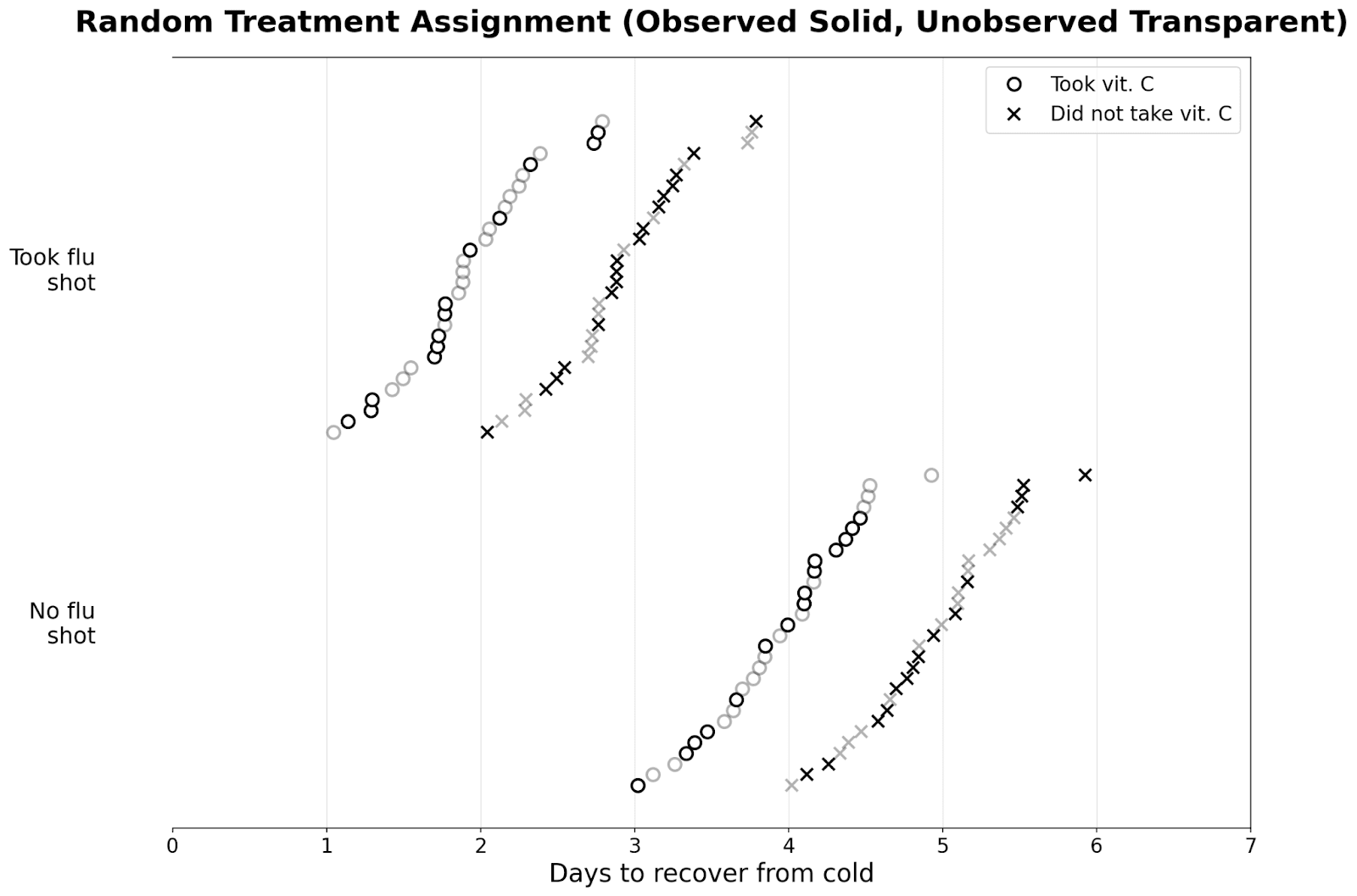
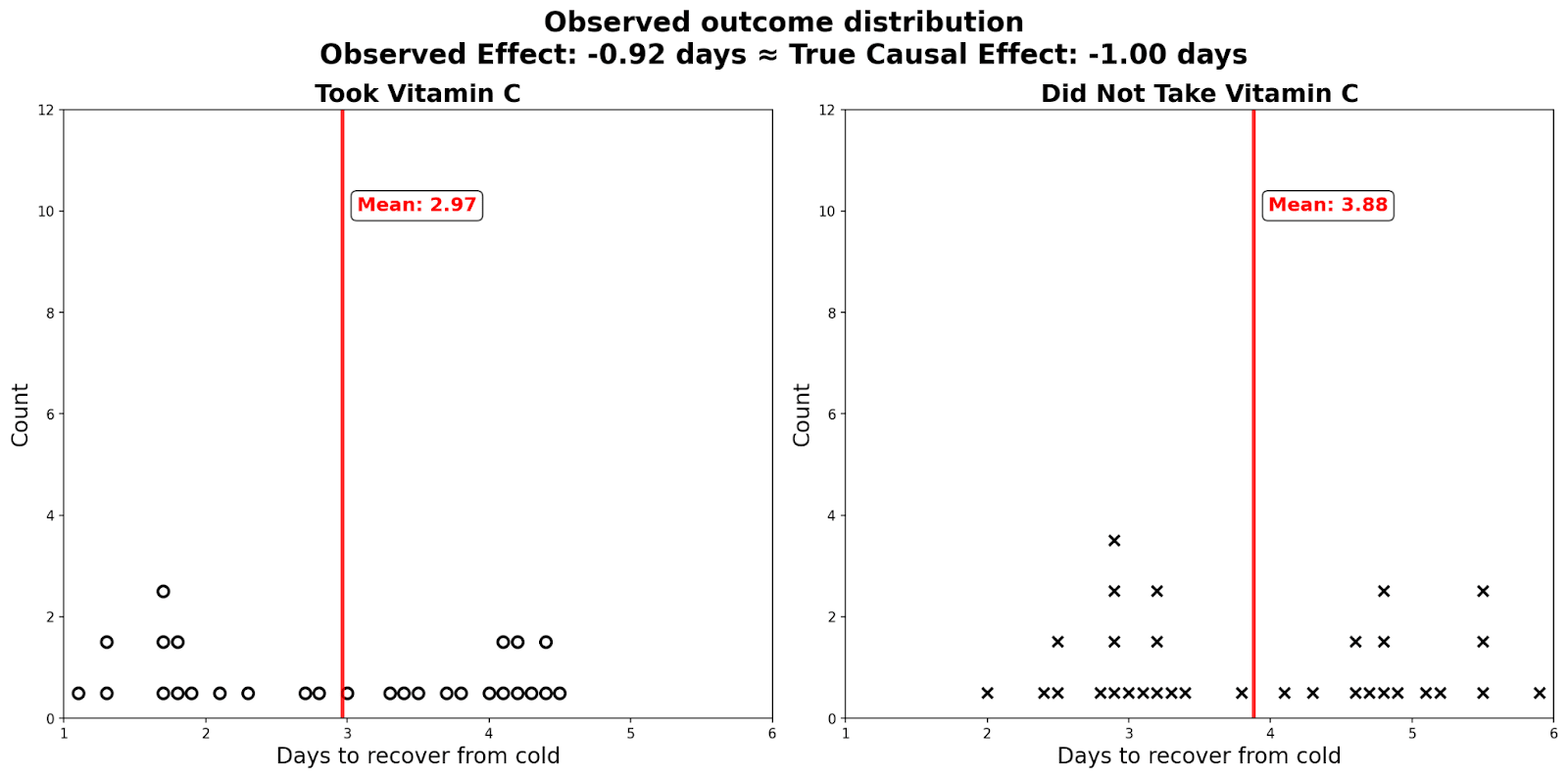
As a result, there is zero selection effect. The observed difference in those who took vitamin C and those who didn’t reveal the true causal effect of the vitamin C pill. I plot the distributions in dot plots below: you can see that there are two modes for people who took/didn't take the flu shot.

Absent experimental data, economists use various other methods to get as close as we can to the experimental ideal. Causal Inference: The Mixtape is a good reference if people are interested in learning more. A particularly cool recent paper tries to directly estimate the selection effect by comparing correlations in observational data with the correlation in randomized experiments.

Advanced Topic: Heterogeneous treatment effect estimation and targeting

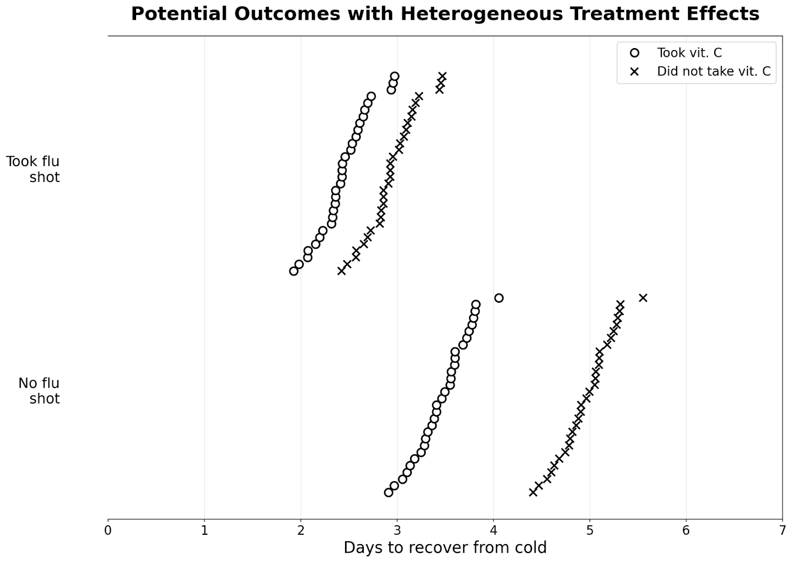
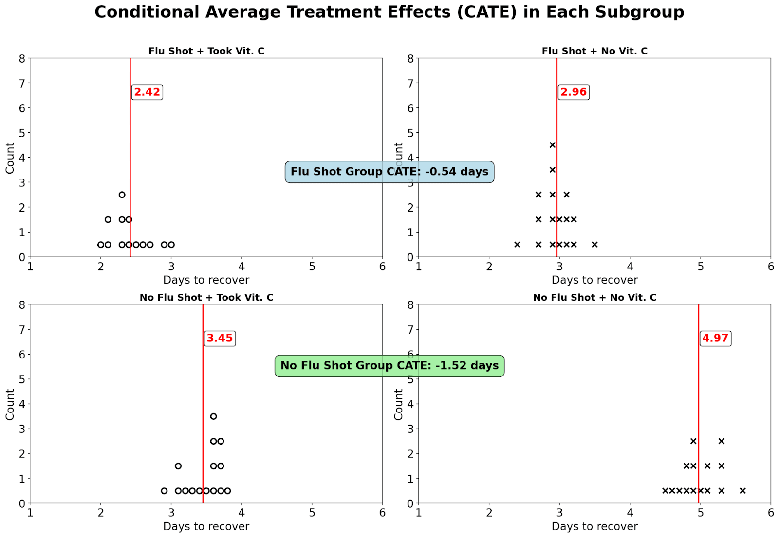
In our previous examples, the effect of our treatment is the same for everyone. However, this might not always be the case. Suppose that the vitamin C pill works much better if you haven’t already taken a flu shot and reduces the length of your cold by 1.5 days, while if you took a flu shot already, the effect is only 0.5 days.

As long as our sample is large and we randomize, we’re likely to get subgroup balance. That is, in any arbitrary subgroup, around half the people would randomly receive the treatment, while half wouldn’t (in reality, we often ensure this by doing block randomization).

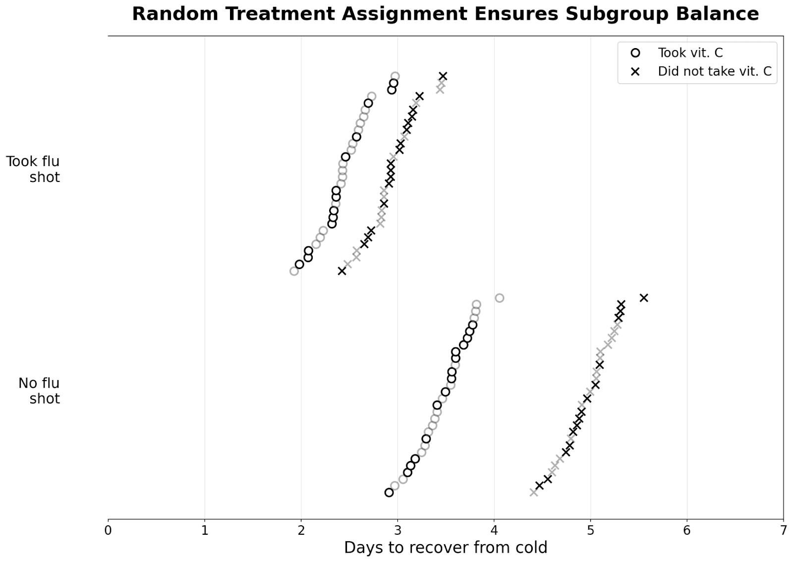
Instead of calculating the average treatment effect by computing the mean days it takes to recover from the cold for those who took the pill and the mean for those who didn’t, we calculate the mean separately for those who took the flu shot and those who didn’t. This gives us the conditional average treatment effect or CATE, which is different from the average treatment effect (ATE) for everyone.

This is the logic behind prioritizing COVID-19 vaccines to vulnerable groups: the treatment effect of the COVID-19 vaccine is larger among some groups compared to others.

In modern-day econometrics, researchers apply machine learning methods to algorithmically discover which subgroups where the treatment effect of an intervention is the largest. In fact, given lots of information on someone’s characteristics, these ML algorithms can predict the treatment effect for an individual–something we could never directly observe. Combined with information on the cost of treatments, causal ML methods allow us to better target our treatment to units where it is the most efficient. This is a lot of what I did when I worked as an economist at Walmart. If you’re interested in learning more, I recommend Susan Athey’s Stanford class, as well as the paper Treatment Allocation Under Uncertain Costs.

Advanced Topic: SUTVA violation and spillover effects

This one is hard to illustrate graphically, but I want to mention it here for completeness. In previous examples, the potential outcomes of a treated unit depend only on its own treatment status and not the treatment status of others: how long it takes for me to recover from the cold doesn’t depend on if someone else took a vitamin C pill. This is called the stable unit treatment value assumption (SUTVA). 

This assumption often does not hold when there are interactions between units. For example, the causal effect of a COVID-19 vaccine on my health depends on whether others around me are vaccinated. If everyone else is vaccinated, then the level of COVID-19 is low. Thus, I’m unlikely to get COVID-19, and the expected effect of the vaccine is low. Similarly, if I get vaccinated from COVID-19, it also helps improve the health outcomes of everyone around me (in expectation).

I'm personally not as familiar with this literature, but those interested in learning more could probably start with Average Direct and Indirect Effects Under Interference and Treatment Effects Under Market Equilibrium.

Conclusion

When we make decisions, we're concerned with cause and effect. To measure causality, we need to know not just what is, but what could be. As we've seen, the core challenge is that we only get to observe one potential outcome and can never simultaneously observe the road taken and the one not taken.

In this post, I introduce a new type of chart to illustrate these potential outcomes. I then use the chart to define causation, correlation, and confounding. Through various examples, I show that correlation does not equal causation and causation does not imply correlation. The charts illustrate how randomized assignment with a large sample minimizes selection effects and helps us recover the causal effect. Finally, I cover two advanced topics: heterogeneous treatment effects and SUTVA violations. 

As Alice, Bob, Carol, and Dan recover from their cold, they ponder what could've happen in a different world, where they made different decisions. 

"What if we all did the exact opposite?" muses Alice, still sniffling slightly. "Would I have recovered in three days without vitamin C?"

"And would I have recovered in two days if I'd taken it?" adds Carol, who's feeling much better now.

Bob sits in the corner, sketching o's and x's on his Walmart receipt for Spring Valley Vitamin C Supplement with Rose Hips Tablets, 500 mg, 100 Count. "You know what the weirdest part is?" he finally says. "Even if the vitamin C did absolutely nothing, I'll probably take it again next time. Just in case."

Acknowledgements: Thanks for feedback from Amanda Gregg, Bill Zhang, Jack Zhang, Jasmine Cui, Joseph Campbell, participants at Less Online, and my younger brother. Claude 4 Opus coded up the graphics for plots with many units (both o4-mini and Gemini 2.5 Pro gave confused responses). Gemini 2.5 Pro and Claude 4 Opus helped with editing. 

1. ^{^}

   See here

2. ^{^}

    I’m mostly drawing from causal inference language used by economists, which seems to be pretty distinct from how computer scientists talk about causality. 

3. ^{^}

   These unobservable confounders are everywhere, and they're especially present when you're comparing people who chose to do something with people who didn't choose to do the thing. I claim that this means you should generally ignore causal conclusions from studies that merely control for observable differences between treated or untreated groups (e.g., that one study on the effect of HRT, almost all studies in nutrition, etc.).

Discuss