通过对以星期几为提示时具有高激活度的特征的解码器方向进行PCA，发现不同大小的稀疏自编码器中存在激活主要在特定星期几的特征组。在最小的SAE中，有一个特征在所有工作日令牌上都强烈激活，而在最大的SAE中，有10个工作日特征，其中3个在所有工作日激活，其余7个分别在一周的某一天激活。

对月份特征进行类似分析，发现最小的SAE有一个单一特征会分裂成许多大致同等重要的特定特征。而对于日历年份，情况更为复杂，在21世纪的一些特征中找到主成分的方法可行，但20世纪的则不行，且在较小的SAE中有一组单一年份特征位于图中心，表明这些主成分无法解释它们的方差。

对所有特征进行PCA，包括多年特征，并对其中四分之一的特征用其前三个激活令牌进行标记，得到一个更具结构性的PCA图。在该图中，日历年份特征明显呈逆时针方向排列。

应用二维UMAP到第二大模型的解码器方向，发现大多数单一年份特征紧密分组，使用聚类算法可找到对应单个年份特征的簇，但绝大多数特征的主成分不可解释。

Published on August 17, 2024 1:16 AM GMT

TL;DR: We demonstrate that the decoder directions of GPT-2 SAEs are highly structured by finding a historical date direction onto which projecting non-date related features lets us read off their historical time period by comparison to year features.

Calendar years are linear: there are as many years between 2000 and 2024, as there are between 1800 and 1824. Linear probes can be used to predict years of particular events from the activations of language models. Since calendar years are linear, one might think the same of other time-based features such as weekday features, however weekday activations in sparse autoencoders (SAEs) were recently found to be arranged in a circular configuration in their top principal components. Inspired by this, we looked into weekdays, months, and most interestingly calendar years from the perspective of SAE feature decoder similarity.

For each group of calendar features, we found interesting patterns of feature splitting between sparse autoencoders of different sizes. For calendar years, we found a timeline direction that meaningfully ordered events, individuals, and concepts with respect to their historical period, which furthermore does not correspond to a principal component of the decoder directions. Finally, we introduce a simple method for finding some of these interpretable directions.

Features at different scales

We started by replicating the weekday results by performing PCA on the decoder directions of features that had high activations when prompted with days of the week, using the same GPT-2 SAEs as in this post, ranging from 768 to 98304 features. In the 768 feature SAE, we found a single weekday feature that activated strongly on all days of the week. In the largest SAE, we found 10 weekday features, 3 of which activated on all days of the week, with the remaining 7 activating on a single day of the week each. 

We found a group of features that activate primarily on specific days of the week by taking the top 20 activating samples for each feature and checking that the max activating token in each of these samples was the specific weekday. We found the first two principal components for this set of features, and projected the features that activate on any day or number of days from all SAEs onto these directions. The labeled features are those that activate on a single day across all SAEs, with the multi-day features unlabeled to maintain legibility.

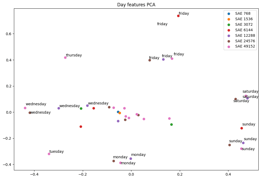
The smallest SAE (blue) has a single feature that activates on all weekday tokens, and lies near the mean of all the weekday features. The largest SAEs learn features for each day of the week, plus additional multi-day features. Across SAE sizes, the single day features form clusters.

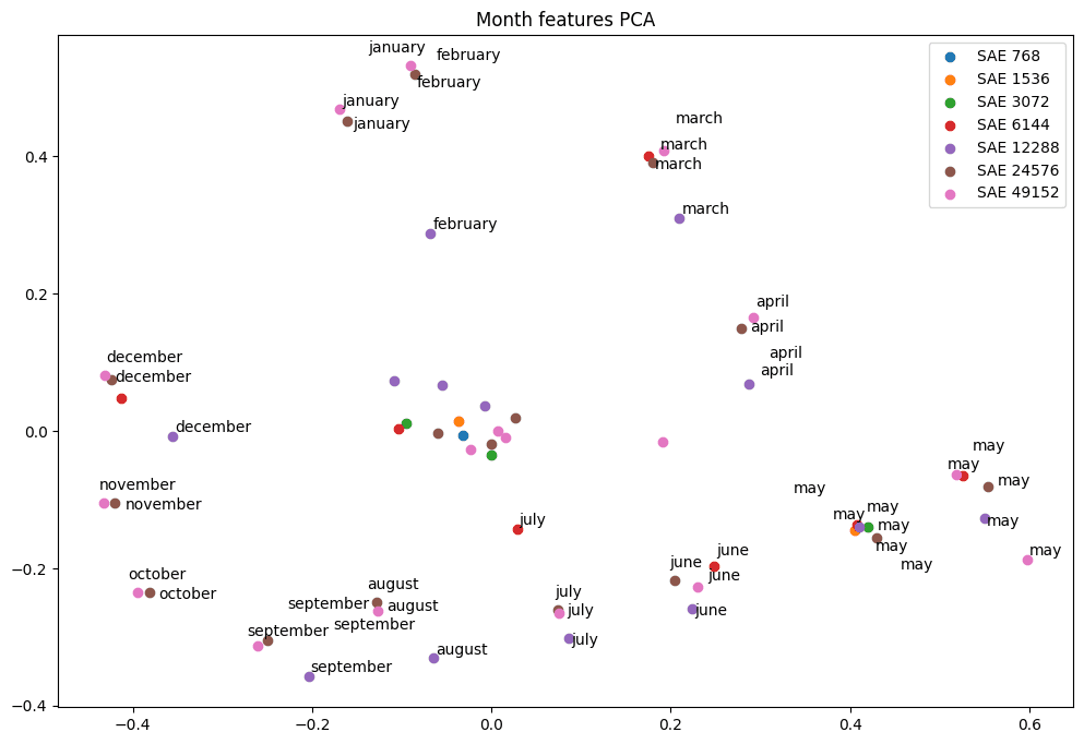
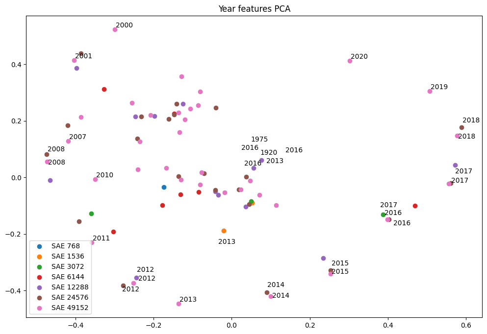
In each of these examples, the smallest SAE has a single feature that splits into many specific features that seem of roughly the same importance. With calendar years, however, the situation is more complex. The same method of finding the principal components for single year features between 1900 and 2020 only succeeds in a few 21st century features, and nothing from the 20th century. There is also a group of single year features in a smaller SAE in the center of the plot, suggesting these principal components do not explain variance in them.

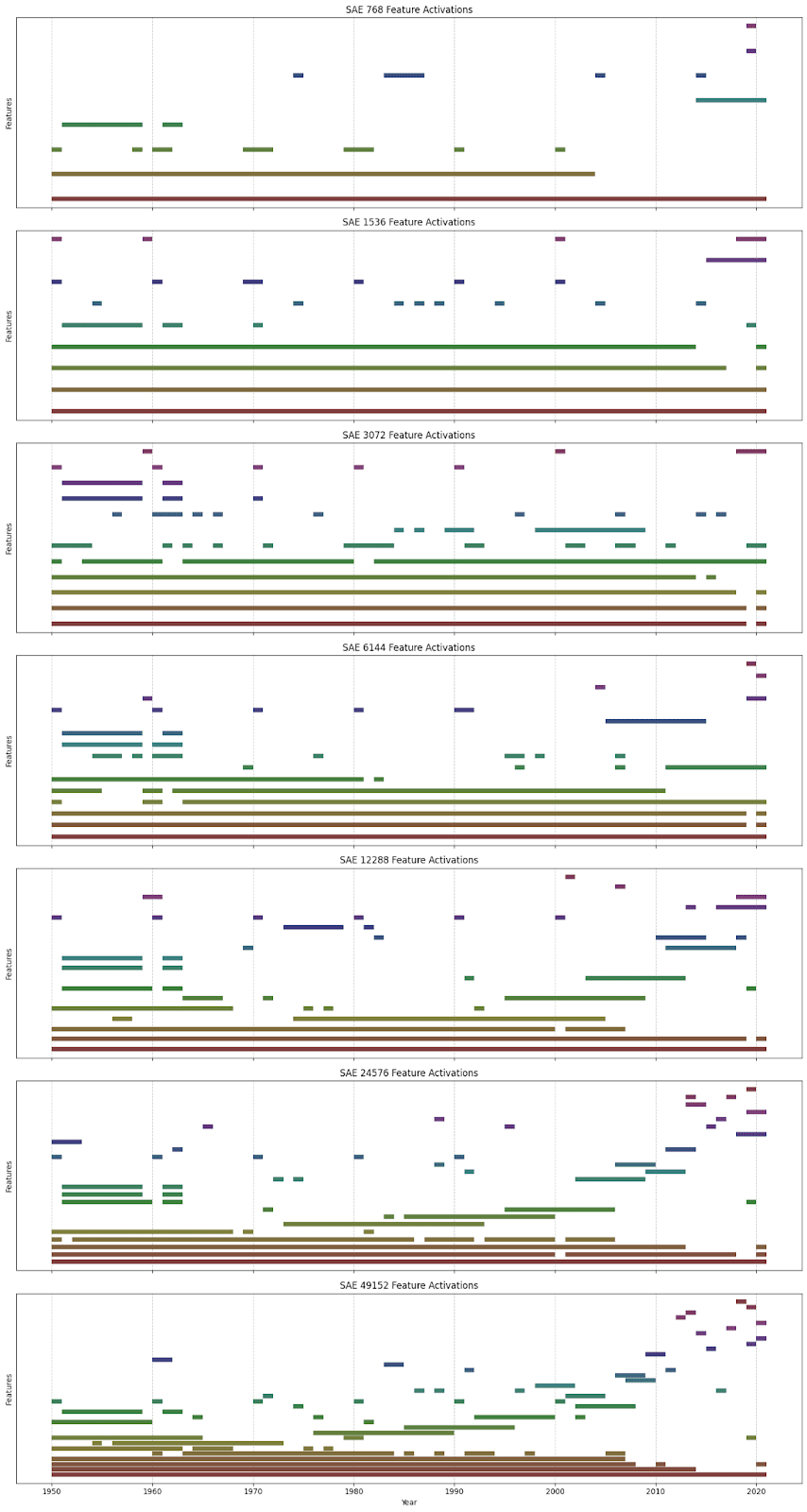
The plot below shows the years for which each of the features is active, with the x-axis being years from 1950 to 2020, the y-axis being separate features, and the colored bars indicating the periods of year for which that feature is active. Only in the largest SAEs do you see more than a few single calendar year features, with most of the features activating on ranges of years, or other patterns such as the start and end of decades.

Performing PCA on all of these features, i.e. including multi-year features, and labeling a quarter of them with their top three activating tokens, results in a more structured PCA plot. In this plot, calendar year features are clearly arranged in a counter-clockwise direction.

Interpreting Principal Components

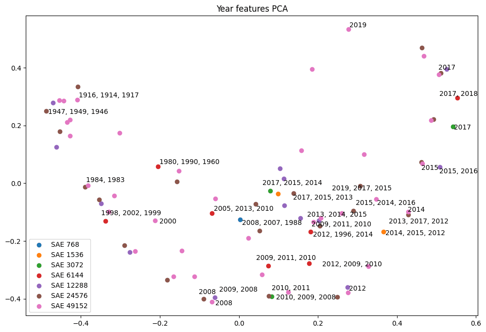
Figure 6 shows a scatter plot of the polar coordinate transformed principal components of calendar year features (i.e. the previous plot with a polar transform applied), with non-year features projected onto these components. The plot is cropped on the x-axis such that 99.5% of the 49152 feature SAE are hidden. The points on the left hand side have been labeled with their top activating tokens, manually selecting a random subsample of features on which we could place a date (i.e. cherry picked but only to the extent that we can estimate a relevant calendar year or period).

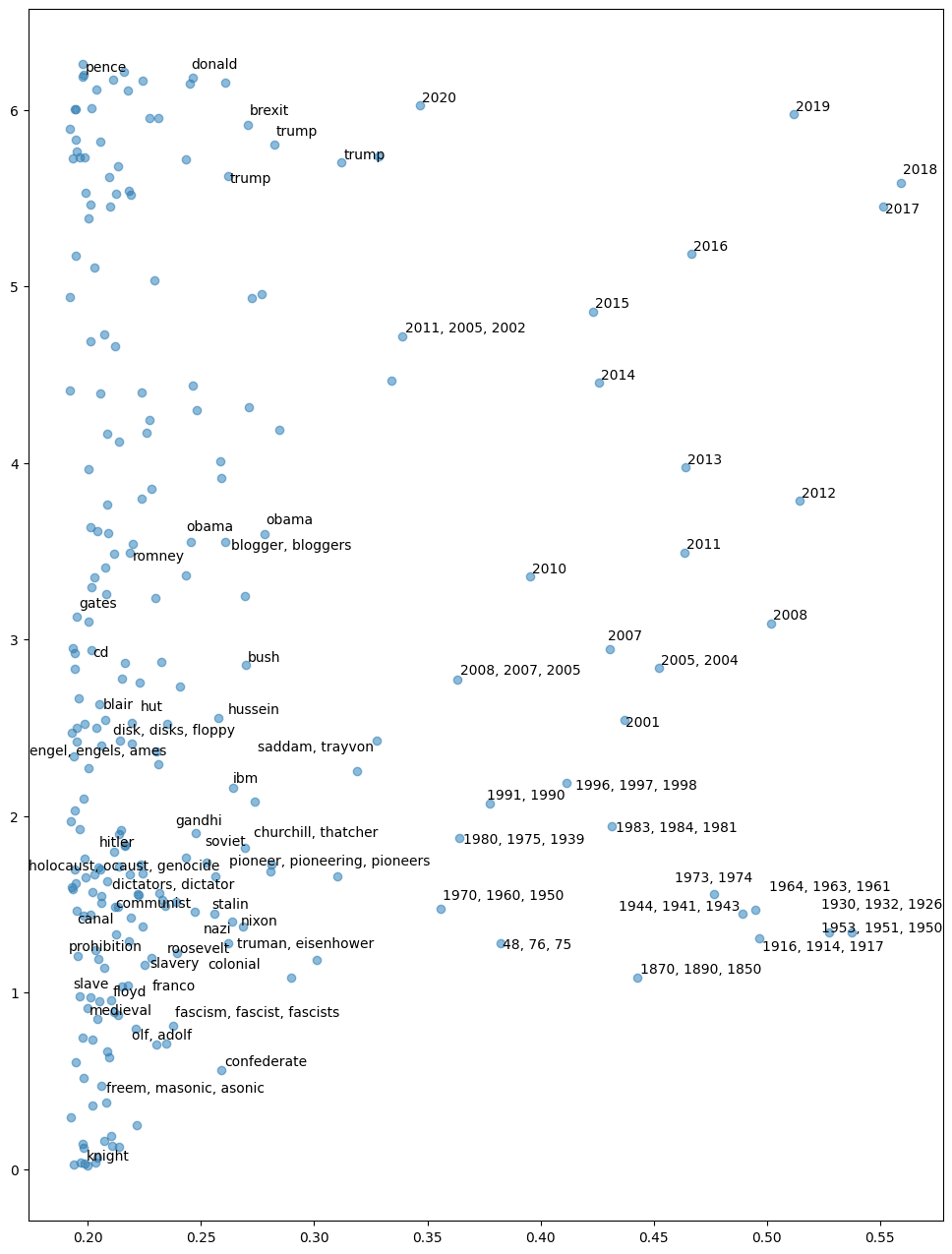
In this plot, the x-axis (i.e. the radius in polar coordinates) seems to represent temporal specificity: the features on the right hand side are individual year features for recent years with a loss of granularity further back in time, those in the middle represent groups of years, and features on the left have nothing directly to do with calendar years. The y-axis (i.e. the angle in polar coordinates), seems to align with increasing calendar year. Not only are the year specific features on the RHS ordered by the year to which they relate, the non-year-specific features on the LHS seem to be sorted by the time period with which they are most associated. A feature for Saddam Hussein precedes features for Barack Obama and Mitt Romney, which in turn precede a feature for Donald Trump.

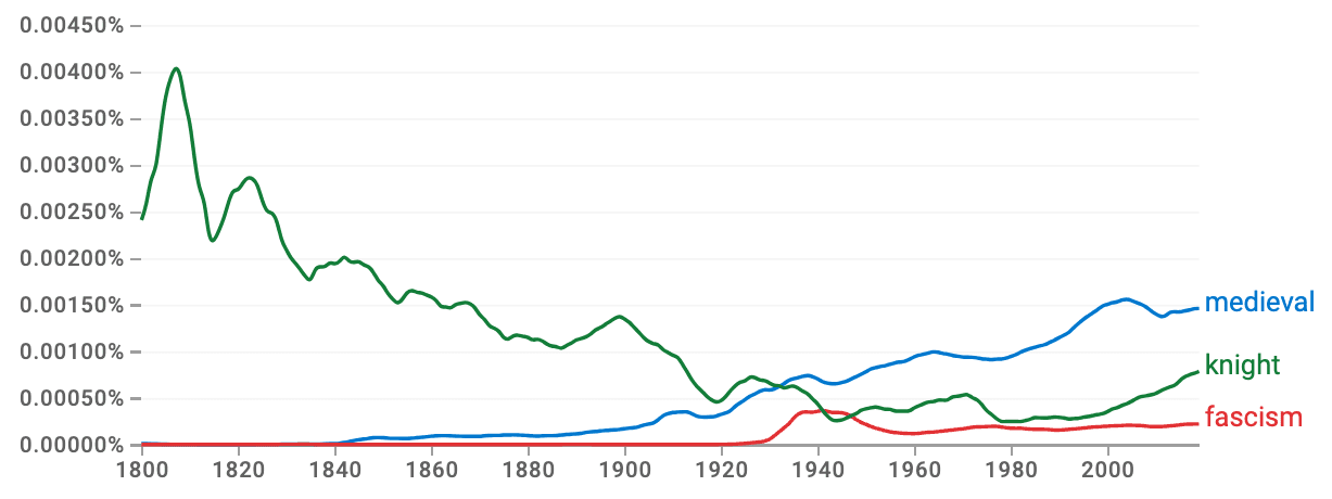
This ordering is clearly not perfect, for example, “medieval” and “fascism” are placed around the same time, whereas “knight” is considerably earlier. However, Google’s ngram frequencies may provide insight into why this might be the case.

Unfortunately, this temporal direction doesn’t correspond to either an SAE feature or a PCA of the entire decoder weight matrix.

Finding Directions

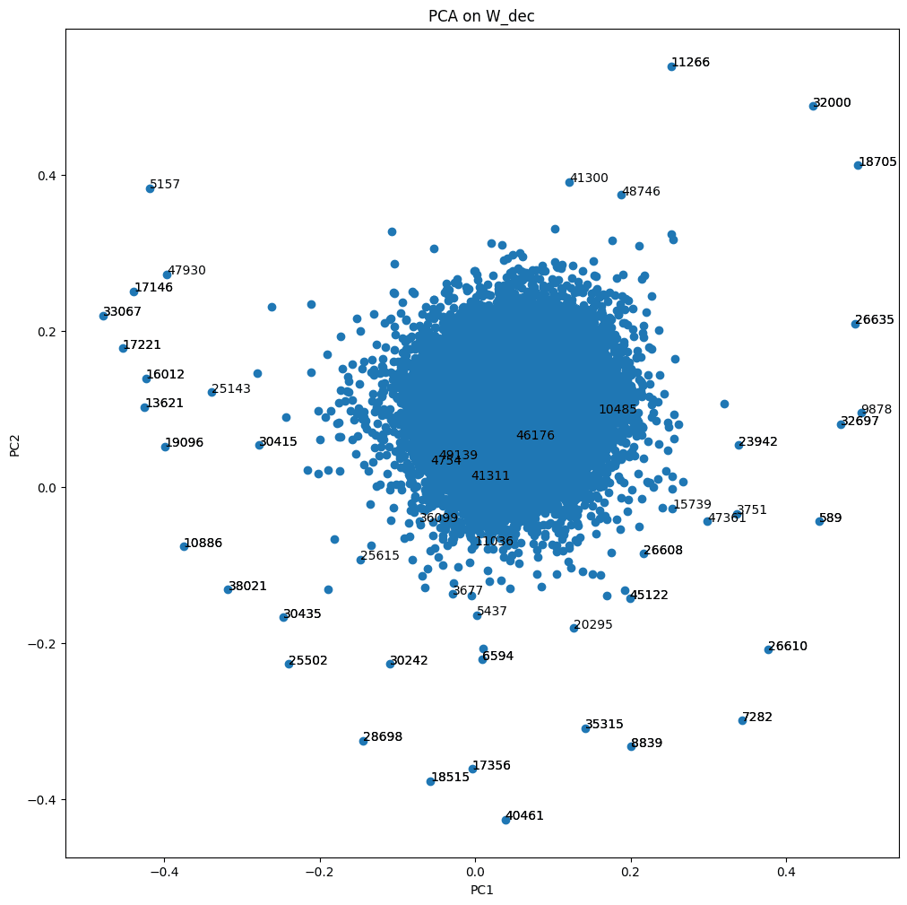
We applied a 2-dimensional UMAP to the decoder directions of our second-largest model and plotted these results below, with the single year features highlighted in red.

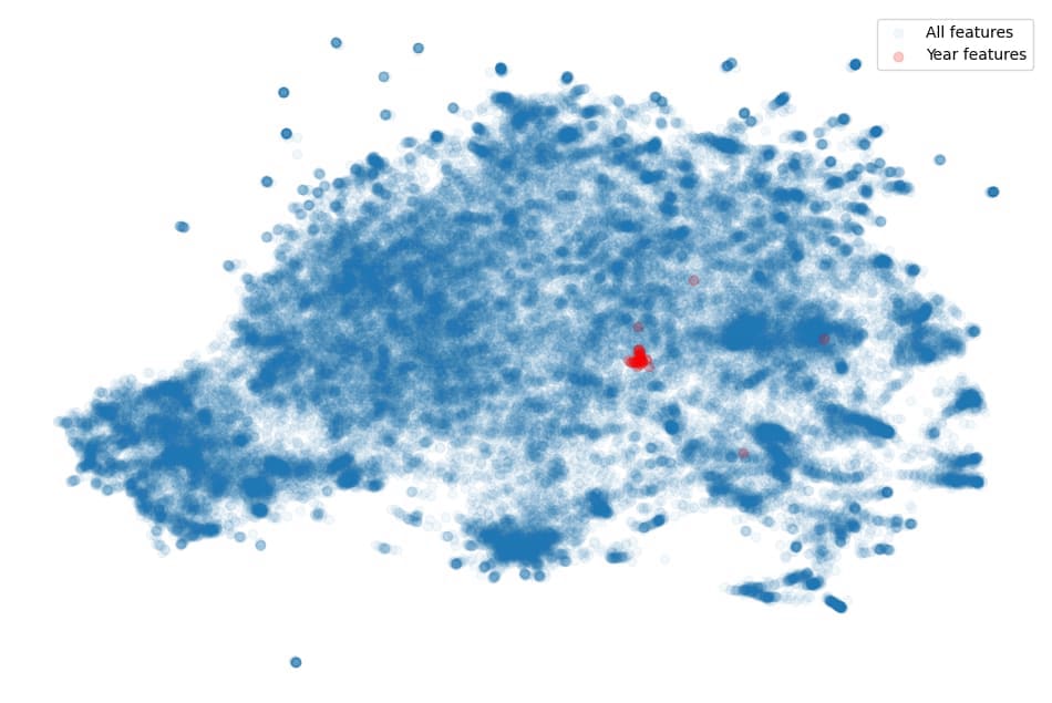
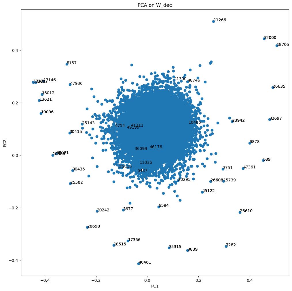
In Figure 8 we see that most of the single year features are all tightly grouped, suggesting it may be possible to find this group of features using a clustering algorithm. Indeed, applying the HDBSCAN clustering algorithm to the 2-dimensional UMAP transformed decoder directions finds a cluster that corresponds to the individual year features. Plotting the projections of all decoder directions onto the first two principal components of this group results in Figure 9, whereas directly using the principal components of the ground-truth year features results in Figure 10. In both cases, the ground-truth year features are labeled, rather than the year tokens, in order to maintain unique labels. Given that the principle components in the left and right plot are very similar, this indicates that we might be able to find these structures in an unsupervised manner.

Other clusters have more or less interpretable principal components, which are displayed below in Figure 10. In these plots, the green points represent cluster features, the red points are points not in the cluster that are furthest from the mean (i.e. how we identified year related features before). These features are labeled with their max activating token.

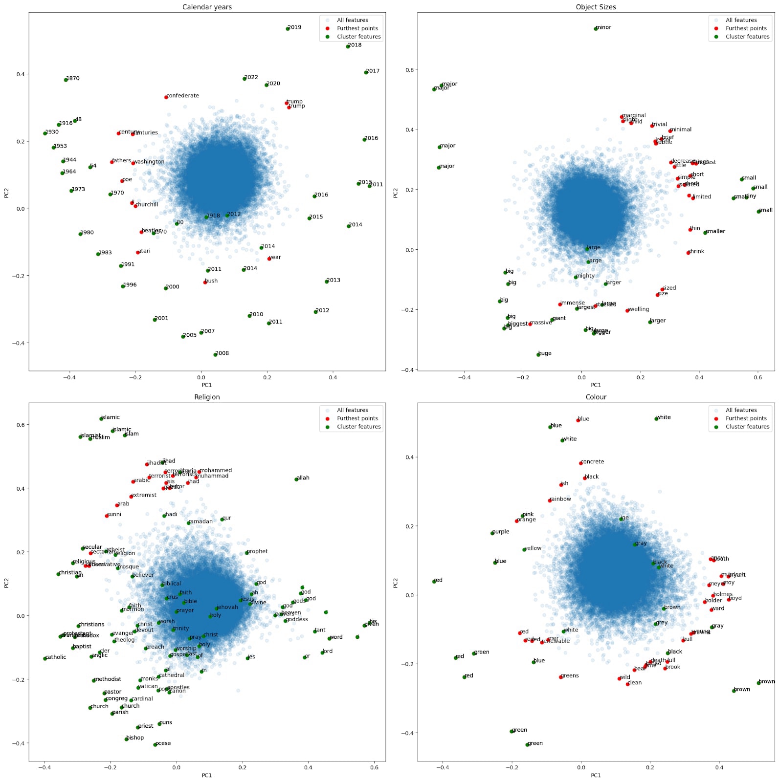
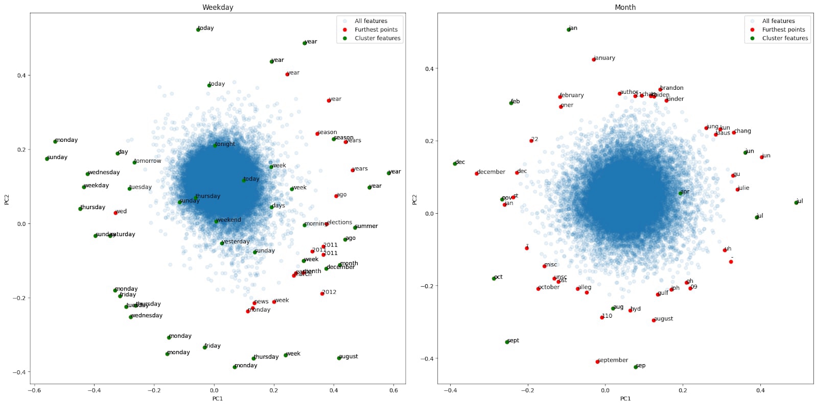
However, the principal components of the vast majority of features were not interpretable (Figure 11). This may be due to many features not having interpretable linear relationships to one another, or our clustering approach just being bad. We have so far spent very little time refining this approach, instead wanting to establish some basic case studies in decoder space structure. We were not able to recover clusters corresponding to weekdays or months with this approach.

Thanks to McKenna Fitzgerald for proofing this post.