本文探讨了并行训练大型模型的两种方法：数据并行和管道并行。数据并行将大型批次分割到多个GPU上，每个GPU计算其子批次的模型输出。管道并行将模型视为管道，每个GPU负责执行管道的一部分，适用于模型过大无法容纳在单个GPU内存中的情况。文章重点分析了管道并行的训练问题，介绍了Dapple和PipeMare等方法，以及用于平衡内存使用和提高效率的管道折叠技巧。

😄 **管道并行：高效的推理，但训练存在挑战** 管道并行将模型分解为多个阶段，每个GPU负责一个阶段，通过将激活传递到下一阶段来实现并行计算。这种方法在推理方面非常高效，但训练时存在挑战，因为需要进行反向传播和权重更新。 由于反向传播需要访问所有激活，导致训练过程中出现“气泡”，即一部分GPU处于空闲状态，降低了效率。Dapple方法通过交织正向和反向传播来减少气泡大小，但无法完全消除。 PipeMare方法通过在权重更新时使用速度估计来近似计算梯度，从而消除气泡。但这种方法可能导致梯度不精确，影响训练效果。

🤔 **解决梯度不精确问题：一种新的权重更新方案** 为了解决PipeMare方法中梯度不精确的问题，本文提出了一种新的权重更新方案。该方案通过交织正向、反向传播和权重更新，确保每次权重更新都使用最新的梯度。 这种方案需要存储前一步的权重，但可以丢弃更早的权重，从而节省内存。虽然这种方法会引入梯度延迟，但可以通过调整学习率来缓解这个问题。

💪 **平衡内存使用：管道折叠技巧** 管道并行中，由于需要存储激活，导致早期层需要比后期层存储更多数据。为了平衡内存使用，本文提出了管道折叠技巧。 这种技巧将管道折叠，使每个GPU处理相同数量的层，并将其配对：第一层与最后一层配对，第二层与倒数第二层配对，以此类推。这种配对方式可以平衡每个GPU的内存使用，确保所有GPU都能有效利用。

🧐 **未来展望：秘密武器和研究方向** 管道并行技术已经存在了一段时间，但许多大型AI实验室可能将其视为“秘密武器”，没有公开发表。未来研究方向可能包括探索更有效、更精确的管道并行训练方法，以及针对不同模型架构和任务的优化技巧。

Published on July 27, 2024 10:40 PM GMT

Epistimic status: Pure speculation; I have 1 GPU, not dozens, so I have no reason to try and implement this stuff myself.

When training large models, we might have many GPUs we'd like to use to speed the process up. This requires a way to parallelize training somehow. Some options here are Data Parallelism and Pipeline Parallelism.

If our model is very large, we might have trouble fitting it into the memory of a single GPU. Pipeline parallelism is convenient in such a case, because it treats the model as a pipeline, where each GPU is responsible for implementing a part of the pipeline. Eg. if the model consists of 64 identical blocks, then we could assign a GPU to each block. Then the activations coming out of each block are passed to the next block. For inference, these activations are the only data that must be communicated between GPUs, which makes pipeline parallelism a very bandwidth-efficient optimization. In order to keep each GPU busy, we must feed in a continuous stream of data, adding more work before the work we previously added makes it through the pipeline.

Data parallelism is where we have a very large batch which we split up across multiple GPUs. Each GPU computes the output of the model on its own sub-batch. We'll mostly focus on pipeline parallelism today, though both methods can be used at once.

Though it's great for inference, pipeline parallelism has some issues for training. Check this article for details, but I'll give a quick overview. The problem is, we have to compute backwards passes, and also weights are continually updated by the optimization algorithm. The need to compute backwards passes introduces a bubble into the system, and the size of the bubble increases with the length of the pipeline. See this figure from the DAPPLE paper:

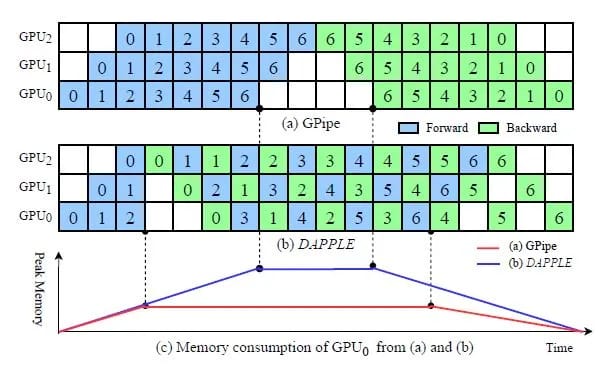
What we can see is that the Dapple method has a much friendlier memory usage than the method originally put forward in GPipe. In hindsight, it's clear that we should try and do the backwards pass as soon as we can after the forwards pass completes, in order to free up all the saved activations. This does get complicated because the amount of work in a backward() is not necessarily the same as the amount of work in a forward(). Let's neglect that issue for now though, and trust that the Dapple paper has provided good methods for dealing with it!

removing the bubble

Dapple doesn't get rid of the bubble, just spreads it out. The origin of the bubble is the desire to cleanly compute a bunch of gradients, then do an optimization step, then repeat the same thing all over again. Each repetition introduces a new bubble. To make the bubble small relative to the middle section where all GPUs are being used, we have to accumulate gradients for a large number of pipeline passes. This means we're forced to multiply the batch size by many times the pipeline length to get a good efficiency. To get rid of the bubble entirely, check out the PipeMare paper. Along with each weight, this paper suggests that we store a velocity estimate for that weight, so that in the backward pass we can get a gradient that is approximately correct.

If you say that approximate correctness is not good enough and you'd like exact correctness, here's a scheme with a similar concept to PipeMare that solves the same problem. (This assumes a maybe unrealistically large amount of synchronization, so we might prefer a scheme like PipeMare in practice.) First, consider the following Dapple-like scheduling scheme (middle): We can see how it is made by interleaving forward passes (left) and backward passes (right).

This is with backwards passes, but without weight updates. Let's say we insert weight updates like so:

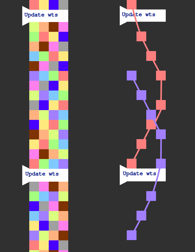
On the right, I've isolated a few forward/backward passes so we can more easily see the causal structure. The spacing of the weight updates is carefully chosen so that each forward/backward pass encloses one weight update. This means that we need to store the weights of the previous time step so that we can keep using them for forward/backward passes that started before the last update. But that's it. We can discard weights from two steps before. The upshot is that by the time we've computed the gradient for the weights at time $t$ the weights are already at version $t+1$. So we must use a gradient descent algorithm something like the following:

$w_{t+1}=w_t-\eta \frac{\partial L}{\partial w_{t-1}}$

where the gradients that are stale by one step.

This is not too bad of a problem. One can study gradient-based optimization methods by looking at their behaviour on a simple loss function like $L=\frac{1}{2}\lambda w^2$. By taking λ to be any complex number, we can then obtain a region of stability in the complex plane. (We have to find the spectral radius of the matrix representing how weights get updated in a full cycle of the optimization algorithm. If it's less than 1, we're in the region of stability. Full stability analysis code at the end of the article.)

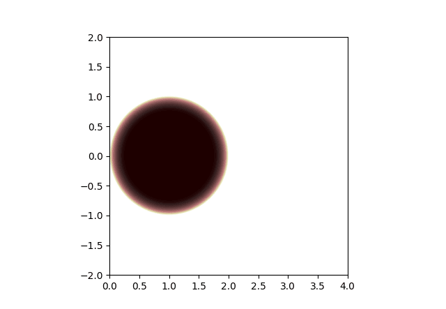
Region of stability for regular gradient descent:

Region of stability for gradient descent with stale gradients:

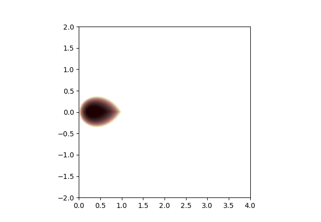
Comparing, we see that the region of stability gets smaller when gradients are stale. So we might have to reduce the learning rate by a factor of 2 or so. But the region of stability is still basically reasonable, it touches the origin, etc.

balancing memory usage by folding the pipeline

There's one more issue to consider: when we compute gradients we need to know the activations from the forward pass. This is the context that gets "saved for backward". If we look at the triangular shape of the forward and backward pass, we can see a bit of a problem: The early layers in the network have to store their activations for much longer than the later layers. Consider the following simple example, a forward and backward pass through 4 identical layers split across two GPUs (dashed line indicates division of work between the two devices).

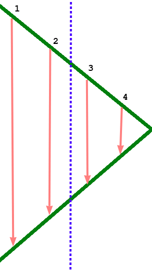
The first device has to store its activations for much longer than the second device, even though it handles the same number of layers. If we consider a longer pipeline with many forward and backward passes being processed at once, the first device in the pipeline is clearly going to run out of memory long before the last one. Though it's hard to avoid the large memory requirements imposed by this, we can at least make sure they are balanced between GPUs. And the trick is a simple one. Just fold the pipeline so that each GPU handles an even number of layers, and the layers are paired together: first with last, second with second last, etc. This balances the memory usage nicely, with memory-hungry early layers being paired with memory-light late layers. This means that a forward pass travels from the first GPU to the last one and back, and a backward pass does the same, for a total of two round trips.

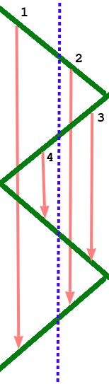
Since new data is continually being processed through the pipeline, there should not be too much imbalance in when the memory is needed.

secret sauce?

Interestingly, this stuff is actually fairly old. PipeMare is from 2020. Though I haven't heard of pipeline folding before, I'm sure it's long since been considered by the big AI labs, and is either in use, or discarded for some even better alternative. I'd guess a lot of these techniques are thought of as "secret sauce" by the big companies, and thus not published, since they provide a competitive advantage.

appendix: stability analysis code

import numpy as npimport matplotlib.pyplot as pltβ = 0.8IMW, IMH = 400, 400EXTENT = [0., 4., -2., 2.]def make_matrix(shape_prefix, lst):  """ broadcast variables to make a matrix """  h, w = len(lst), len(lst[0])  ans = np.zeros(shape_prefix + (h, w), dtype=complex)  for i in range(h):    for j in range(w):      ans[..., i, j] = lst[i][j]  return ans  def A_sgd(λ):  lr = 1.  return make_matrix((IMW, IMH), [[1. - lrλ]])def A_polyak(λ):  lr = 1. - β # corrected LR for momentum method  return make_matrix((IMW, IMH), [    [1. + β - lrλ, -β],    [1.,             0]])def A_nesterov(λ):  lr = 1. - β # corrected LR for momentum method  Q = 1. - lrλ  return make_matrix((IMW, IMH), [    [βQ, Q - 1.],    [βQ, Q]])def A_stale_sgd(λ):  lr = 1.  return make_matrix((IMW, IMH), [    [1., -lrλ],    [1.,  0.]])def get_max_eigenvalue_magnitude(mat):  vals = np.linalg.eigvals(mat)  return np.absolute(vals).max(-1)if name == "main":  X, Y = np.meshgrid(np.linspace(EXTENT[0], EXTENT[1], IMW), np.linspace(EXTENT[2], EXTENT[3], IMH))  λ = X + 1j*Y  for A_fn in [A_sgd, A_stale_sgd]:    A_1 = A_fn(0.01)[0, 0] # specifically for λ = 0.1, what is the convergence rate?    print(get_max_eigenvalue_magnitude(A_1)) # did we correctly tune lr for momentum methods?    A = A_fn(λ)    color = np.minimum(1., get_max_eigenvalue_magnitude(A)**20)    plt.imshow(color, cmap="pink", extent=EXTENT)    plt.show()

Discuss