本文深入探讨了概率实验的概念，并以此为基础推导了条件概率和事件的定义。作者指出，在实际应用中，条件概率往往比联合概率更为基础，而条件化本身是概率论的核心。通过将概率实验视为一系列可迭代的试验，并引入条件化函数，文章清晰地展示了如何从原始实验过渡到条件概率实验，从而解释了事件集合与事件命题之间的联系。文章还通过代码示例和反例，阐述了条件化的必要条件，以及概率如何在条件化过程中重新分配，为理解概率论提供了新的视角。

💡 **条件化是概率论的基石**：文章认为，与传统上从联合概率推导条件概率不同，实际应用中条件概率更为基础。作者提出，条件化本身才是概率论的核心，它允许概率理论应用于认识论，即知识状态的更新。通过将概率实验视为一个可以被“条件化”的过程，可以更直观地理解概率的运作。

🎲 **概率实验与条件化**：作者将概率实验定义为一个将自然数映射到可能结果的函数，例如掷骰子。条件化则是一个二阶函数，将一个概率实验转化为另一个条件概率实验，其结果是原始实验结果的一个子集。例如，从一个标准的D6骰子实验（结果为{1,2,3,4,5,6}）进行“偶数条件化”，得到一个新的实验（结果为{2,4,6}），这比传统的通过联合概率计算条件概率更透明。

💬 **事件的本质是条件命题**：文章解释了事件集合与事件命题之间的联系。一个事件命题可以被看作是对实验每一次迭代结果的一个布尔函数，即判断该结果是否满足某个条件。当这个条件是关于结果属于某个特定集合时，就与事件集合直接对应。即使条件不那么明确（例如“75%可能为偶数”），也可以通过更精细化的样本空间或直接的条件化函数来处理，而无需预先修改样本空间。

📈 **概率的重新分配**：文章阐述了在条件化过程中，概率是如何在实验结果之间重新分配的。原始实验中所有可能结果的概率总和为1。当进行条件化时，那些不满足条件的迭代所携带的概率会被重新分配给满足条件的迭代。一个事件的概率越低（即在原始实验中越罕见），在条件化时被重新分配的概率就越多，这解释了条件概率的计算方式。

🔑 **概率论基础的重塑**：通过“概率实验”和“条件化”的概念，作者成功地从逻辑上重新构建了概率空间（Ω,F,P）的三个基本要素：样本空间、事件和概率测度。文章强调，一个陈述只有在对实验的每次迭代都有明确的真假值，并且在无限多的迭代中为真时，才能被视为一个事件，并因此具有概率测度。这为解决困扰哲学家多年的概率理论问题提供了新的视角。

Published on July 25, 2025 6:07 AM GMT

In the previous post we've established the notion of a probability experiment and had a brief glance how it can be used to describe knowledge states and Bayesian updates. Now let's talk about it in more details and see how all our standard probability theoretic concepts can be derived from it.

And as a starting point, let's talk about conditionalization.

Usually to do it, we're required to perform some preparations beforehand:

Define Sample Space $\Omega$Define Event Space $F$Define Probability function  $P:F\to [0;1]$

Define conditional probability through probability of joint intersection of events:

 $P\left(A|B\right)=P(A\cap B)/P\left(B\right)$

As far as mathematical formalism goes, this is fine. But if we look at a typical case in the real world, this is backwards. We almost never start knowing the probability of joint intersection of events, from which we calculate conditional probability. Usually we know some conditional probability $P\left(A|B\right)$ and need to calculate conditional probability $P\left(B|A\right)$, for which we apply Bayes' Theorem.

Consider the standard example:

1% of women at age forty who participate in routine screening have breast cancer. 80% of women with breast cancer will get positive mammograms. 9.6% of women without breast cancer will also get positive mammograms. A woman in this age group had a positive mammogram in a routine screening. What is the probability that she actually has breast cancer?

We didn't get our P(PositiveMammogram|Cancer)=80% from knowing the rate of Positive Mammogram in a general female population at the age of forty. Instead we get this conditional probability from the data directly. From all the cases where the woman at the age of forty, participating in routine screening, actually happened to have cancer we check which ratio had a positive result on a mammogram.

So, in practice, it's conditional probability that appears more fundamental than probability of join intersection. But what really is fundamental is conditionalization itself. It's a cornerstone of probability theory, which allows it to be applicable to epistemology in the first place. How comes we only talk about conditionalization through some measure function?

With the notion of probability experiment, let's define conditional probability and conditionalization itself in a straightforward manner.

Conditional Probability Experiment

Consider a D6 Roll probability experiment.

$D6R:N\to \{1,2,3,4,5,6\}$

also generalizable as

$Sample\left(6\right)$

It corresponds to a knowledge state, according to which a D6 was rolled and there is no other information about which side is the top one.

What happens when we learn that the outcome of the dice roll is even? Previously we were equally uncertain between six different outcomes, now we are equally uncertain between three even ones. There is now a different probability experiment corresponding to our knowledge state - Even D6 Roll:

$ED6R:N\to \{2,4,6\}$

$Sample\left(3\right)$

So we say that ED6R is a conditional probability experiment of D6R

And we define Even Conditionalization $EC$ as a second order function that turns D6R into ED6R:

$EC:D6R\to ED6R$

In a general case:

CPE is a conditional probability experiment of PE iff

PE is a probability experiment
$PE:N\to \Omega$
$P{E}_i={\omega }_k\perp P{E}_j={\omega }_l\forall i\ne j\forall k,l$CPE is a probability experiment:
$CPE:N\to {\Omega }^{\prime }$
$CP{E}_i={\omega }_k\perp CP{E}_j={\omega }_l\forall i\ne j\forall k,l$Codomain of CPE is a subset of Codomain of PE:
${\Omega }^{\prime }\subseteq \Omega$

then C is a conditionalization of PE into CPE iff

$C:PE\to CPE$

Examples of Conditionalization

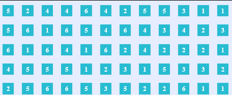
Consider a sequence of outcomes of our unconditional experiment D6R, which we can get by rolling a D6 die multiple times:

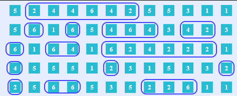
What happens with this sequence when we apply even conditionalization? All the outcomes that satisfy the condition are preserved, while those who do not are thrown away.

We can treat this as executing a simple program that iterates over the outcomes of the experiment, accepting the iterations that satisfy the condition of evenness and rejecting all that don't. And from the accepted iterations the conditional probability experiment is produced.

def even_conditionalization(D6R):   for outcome in D6R:     if outcome in {2, 4, 6}:            yeild outcome       ED6R = even_conditionalization(D6R)

Here, I hope, you can see the beauty of our approach to conditionalization. Instead of two values of a measure function we now have a transparent belief updating algorithm.

Another example is trivial or identity conditionalization, where all the iterations of the experiment are preserved. 

def identity_conditionalization(D6R):  for outcome in D6R:     if outcome in {1, 2, 3, 4, 5, 6}:           yeild outcome       D6R = identity_conditionalization(D6R)

According to our definition any probability experiment is a conditional probability experiment of itself, and therefore

$I:D6R\to D6R$

is a valid conditionalization. We can have a different algorithm for trivial conditionalization, for instance:

def identity_conditionalization(D6R):    for i, outcome in enumerate(D6R):       if i%2 == 0:            yeild outcome       ED6R = even_conditionalization(D6R)

Here we preserve only every second iteration of the experiment. But, as it doesn't affect the ratio of the outcomes throughout the experiment, this is still identity conditionalization. 

Counterexamples

Now let's consider some counter-examples.

Not every modification of a probability experiment is a conditionalization. For instance, 

D6R→ ED6R'

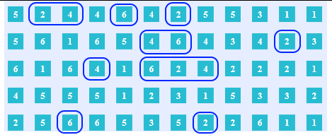
Here the outcomes are preserved based on which outcomes were before. As a result, values of ED6R' are not statistically independent. Therefore, ED6R' is not a probability experiment at all and, therefore, not a conditional probability experiment of D6R.

Another counter-example is a modification of probability experiment that does something beyond filtering some of the outcomes, like adding new outcomes or replacing some outcomes with different ones. 

And of course if we reject all the trials of the experiment, getting as a result a function whose domain is an empty set, this is also not a conditionalization, as probability experiments' domain is the set of natural numbers.

Event-Sets and Event-Propositions

Now let's talk about events. Historically there is a weird mishmash regarding this term. Initially event-space was defined as a sigma algebra over the sample space and therefore events were defined as sets of possible outcomes.

But then some authors started talking about event-spaces that consisted of statements that can be either true or false. And curiously enough, both ways to reason about probability theory produced the same results. How come? Why do propositions work the same way as sets?

With our new understanding of conditionalization in mind, we can solve this mystery. Let's look again at the code of the even_conditionalization function. More specifically, the third line:

if outcome in {2, 4, 6}:

Here we have a condition which each trial can either satisfy or not. And this condition is about membership in a set of the outcomes of the experiment. After conditionalization, this set becomes the sample space of the conditional probability experiment. 

So we are going to say that this set:

$\{2,4,6\}$

is the event-set of conditionalization EC

and the conditional statement "The outcome of this iteration of experiment is even", that can be either true or false for any iteration of the experiment:

$D6R_i\in \{2,4,6\}$

is the event-proposition. 

In a simple case, where a proposition is solely about a membership of an outcome of a trial in a set of outcomes of a probability experiment, the situation is clear. We have a direct isomorphism between sets of outcomes and such propositions. So no surprise that both approaches to events produce the same results. But what about more nuanced cases?

More Granular Events

Consider this. Suppose we didn't learn for sure that the outcome is even. We only became 75% confident that it is so. As a result no outcomes from the sample space of the initial experiment are eliminated, some simply became rarer. How do we express such an event in terms of sets?

The standard practice is to make the sample space more granular. We modify it from

$\{1,2,3,4,5,6\}$ to $\{1_1,1_2,2,3_1,3_2,4,5_1,5_2,6\}$

therefore, changing^[1] the whole experiment from

$Sample\left(6\right)$  to $WeightedSample(9,\{1/12,1/12,1/6,1/12,1/12,1/6,1/12,1/12,1/6\left\}\right)$

And then with this more granular sample space we can say that the proposition

"The outcome of this iteration of experiment is 75% likely to be even"

is a proposition about a membership in a set $\{1_1,2,3_1,4,5_1,6\}$:

$D6R_i\in \{1_1,2,3_1,4,5_1,6\}$

And as a result of conditioning on such event we get a probability experiment

$WeightedSample(6,\{1/12,1/4,1/12,1/4,1/12,1/4\left\}\right)$

In principle, we can do this for any proposition about the outcomes of the trials, constantly refining the sample space as needed and therefore preserving the isomorphism between sets and propositions. But in practice, such retroactive modifications every time we need to express a more nuanced event are very inconvenient.

Thankfully, our notion of probability experiment and conditionalization provides a better option. Ultimately what we want, is to go from

 $Sample\left(6\right)$ 

to 

$WeightedSample(6,\{1/12,1/4,1/12,1/4,1/12,1/4\left\}\right)$

So all we really need is one conditionalization

$E075C:Sample\left(6\right)\to WeightedSample(6,\{1/12,1/4,1/12,1/4,1/12,1/4\left\}\right)$

def even_075_conditionalization(D6R):    for i, outcome in enumerate(D6R_mod):        if outcome in {2, 4, 6}:           yeild outcome        elif i%2 == 0          yeild outcome            E075D6R = even_075_conditionalization(D6R)

And there is no need to granularize the sample space beforehand. 

Necessary Condition

Now let's refactor the code a bit:

def satisfy_condition(i, outcome):    if outcome in {2, 4, 6}:        return True    elif i%2 == 0        return True    else        return False                def even_075_conditionalization(D6R):    for i, outcome in enumerate(D6R_mod):        if satisfy_condition(i, outcome):            yeild outcome

And see that event-proposition can be expressed as a boolean function of trials:

$Even{t}_p:(i,PE[i\left]\right)\to \{True,False\}$

From it we have a necessary condition. To be an event-proposition in a probability experiment, a statement has to:

Have a coherent truth value in every trialBe True on some countable subset of trials

Otherwise, we won't be able to perform conditionalization and get a valid conditional probability experiment. Or, in other words, if the condition for our belief updating is ill-defined we can not execute the algorithm.

Probability and Conditional Probability

So every conditionalization has a conditional statement, also known as event-proposition.

In every iteration of the probability experiment conditional statement has a well-defined truth value and is true in an infinitely many trials. But some statements are true more often than others. And we would like to somehow be able to talk about it.

Therefore - the concept of probability. It's a measure function of truthfulness of a statement throughout the whole experiment. Let N be the number of iteration of experiment and T - the number of iterations in which the statement is true. Then we define probability of a statement as:

$P\left(Statement\right)=Li{m}_{N\to \infty }T/N$

And what about conditional probability? Well, basically the same thing. Conditional probability is simply probability of a conditional probability experiment.

$P\left(Statement|C\right)=Li{m}_{N_c\to \infty }{T}_c/N_c$

Where $N_c$ is the number of iterations of conditional probability experiment and $T_c$ is the number of iterations of conditional probability experiment in which the statement is true.

Let's look again at our example with a D6 Dice Roll:

Consider a proposition "The outcome of the roll is 4". Its unconditional probability is:

P(4) ~ 9/60 ~ 1/6

Meanwhile, conditionally on the fact that the outcome is even:

P(4|2 xor 4 xor 6) ~ 9/31 ~ 1/3  

Which is, once again, exactly how we deal with conditional probability in practice. See the mammogram example from the beginning of the post.

A helpful way to look at it is to think that every iteration of the experiment holds an infinitesimal amount of probability, which adds up to 1, similarly to how an infinite number of dots can add up to a line segment with length 1. 

Now what happens to probability under conditionalization?  At first all of it is evenly spread among all the iterations of the initial probability experiment. Then after conditionalization, it has to be spread among all the iterations of the conditional probability experiment. So all the probability of the iteration of the initial experiment for which the conditional statement is False, is evenly redistributed among the iterations of the experiment for which the conditional statement is True.

Lower probability of the conditional statement means that it's True for less iterations of the initial experiment and, therefore, more probability is reallocated on conditionalization. To reallocate 1-p fraction probability on conditionalization, its conditional statement has to have probability p in the initial experiment.

Conclusion

And so we've established all the basic concepts of probability theory through the notions of experiments and their conditionalizations. We have our outcomes, events and probability measures - the three elements of the probability space  $(\Omega ,F,P)$. And therefore all the standard math applies.

However, now we've logically pinpointed  the relation between the map and the territory more accurately. While previously we could only talk about overall properties of the probability spaces, we can now say something about whether the particular model is appropriate to the real world process. We've established several core rules:

The Sample Space consists of the unique outcomes of the probability experiment, which is an approximation of some process in the real world to the level of our knowledge about it.A statement in a natural language is an event only if it is a well-defined function of trials: it's True in some countable subset of the iterations of the experiment and False in every other iteration of the experiment.Probability is a function of events. Any statement that is an event has a probability measure. If some statement isn't an event, then it doesn't have a probability measure.If statement has probability p in an experiment it means that p is the ratio of trials in which this statement is true in this experiment and vice versa.The rarer is the event, the more probability will be redistributed, during conditionalization on it.

If these rules appear very obvious to you, that's because they are. And yet, it's important to state them explicitly. Because, following them and noticing when someone fails to, is enough to solve every probability theoretic problem that have been confusing philosophers for decades.

1. ^{^}

   Notice, that this isn't conditionalization, as the resulting sample space is not a subset of the initial one.

Discuss