
Cold start in recommendation systems goes beyond just new user or new item problems—it’s the complete absence of personalized signals at launch. When someone first arrives, or when fresh content appears, there’s no behavioral history to tell the engine what they care about, so everyone ends up in broad generic segments. That not only dampens click-through and conversion rates, it can drive users away before a system ever gets a chance to learn their tastes. Standard remedies—collaborative filtering, matrix factorization, or popularity lists—lack the nuance to bridge that signal gap, and their one-size-fits-all suggestions quickly feel stale. Imagine, instead, if you could generate detailed interest profiles from day one. By tapping into large language models (LLMs) for zero-shot reasoning, you can synthesize rich, context-aware user and item embeddings without waiting for weeks of interaction data—turning a cold start into a warm welcome.
In this post, we demonstrate how to use vLLM for scalable inference and use AWS Deep Learning Containers (DLC) to streamline model packaging and deployment. We’ll generate interest expansions through structured prompts, encode them into embeddings, retrieve candidates with FAISS, apply validation to keep results grounded, and frame the cold-start challenge as a scientific experiment—benchmarking LLM and encoder pairings, iterating rapidly on recommendation metrics, and showing clear ROI for each configuration.
Solution overview
We build our cold-start solution on Amazon EC2 Trainium chips. To streamline model deployment, we use DLCs with the AWS Neuron SDK, which installs Neuron-optimized PyTorch modules and includes the latest AWS Trainium drivers and runtime pre-installed.
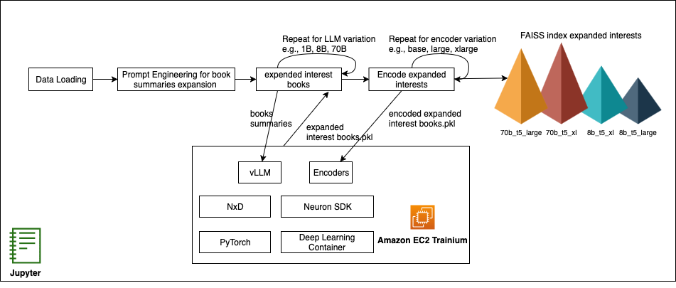
Figure : Cold-start recommendation pipeline on AWS Trainium with vLLM & NxD
Sharding large models across multiple Trainium chips is handled by the distributed library used by Neuron, NeuronX Distributed (NxD), which integrates seamlessly with vLLM. NxD manages model partitions across multiple instances with minimal code changes, enabling parallel inference of even 70B parameter LLMs. This combination—Trainium chips, Neuron Tools, and vLLM—gives machine learning (ML) engineers a flexible, cost-efficient, production-ready solution for experimenting with different LLM and encoder configurations and delivers rapid iteration on recommendation quality metrics without modifying core model code.
In the next section, we orchestrate our experiments in a Jupyter notebook—providing a reproducible, end-to-end workflow from loading data and engineering structured prompts to generating embeddings and retrieving candidates with FAISS—complete with interactive charts to visualize recommendation performance. Then, in the production deep-dive, we walk through a reference implementation that packages your Neuron-optimized LLM and encoder as DLC images and deploys them on Amazon Elastic Kubernetes Service (Amazon EKS) with autoscaling, so your inference layer automatically adapts to demand while optimizing cost and performance.
Expanding user interest profiles with LLMs
In this post, we use the Amazon Book Reviews dataset (mohamedbakhet/amazon-books-reviews) from Kaggle, which provides real-world user reviews and metadata for tens of thousands of books. This rich collection lets us simulate cold-start scenarios—where a brand-new user has only a single review or like—and evaluate how well our interest expansions, powered by distilled versions of Meta’s Llama 8B and 70B models, generate rich user profiles. We use an LLM to enrich a new user’s profile from minimal initial data. For example, if a user has only reviewed one science fiction novel, the LLM infers related subtopics—such as galactic empires, cyberpunk dystopias, or space exploration—that the user is likely to enjoy. We use structured prompts that embed the user’s existing activity into a concise instruction to verify consistency and relevance, as demonstrated in the following example:
By constraining the LLM’s output format—asking it to return a JSON array of topic keywords—we avoid free‑form tangents and obtain a predictable list of interest expansions. Modern generative models, such as Meta’s Llama, possess broad domain knowledge and human‑like reasoning, enabling them to connect related concepts and serve as powerful cold‑start boosters by inferring deep user preferences from a single review. These synthetic interests become new signals for our recommendation pipeline, allowing us to retrieve and rank books from the Amazon Reviews collection even with minimal user history. You can experiment with Llama variants ranging from one‑billion to seventy‑billion parameters to identify which model yields the most discriminative and relevant expansions. Those findings will guide our choice of model for production and determine the size and scale of the Amazon EC2 Trainium and Inferentia instances we provision, setting us up for live user A/B tests to validate performance in real‑world settings.
Encoding user interests and retrieving relevant content
After we have our expanded interests, the next step is to turn both those interests and our catalog of books into vectors that we can compare. We explore three sizes of the Google T5 encoder—base, large and XL—to see how embedding dimensionality affects matching quality. The following are the steps:
- Load the encoder for each size Encode book summaries into a single NumPy matrix and normalize it Build a FAISS index on those normalized vectors for fast nearest‑neighbor search Encode the expanded interest text the same way and query FAISS to retrieve the top k most similar books
You can compare how each encoder scale affects both the average FAISS distance (that is, how far apart your interest is from the content) and the actual recommended titles. Swapping in a different encoder family—such as SentenceTransformers—is as straightforward as replacing the model and tokenizer imports.
Measuring and improving recommendation quality
Now that we’ve generated FAISS indexes for every LLM‑encoder pairing and computed the mean distance between each expanded interest query and its top 10 neighbors, we know exactly how tightly or loosely each model’s embeddings cluster. The following chart shows those average distances for each combination—revealing that 1B and 3B models collapse to almost zero, while 8B and 70B models (especially with larger encoders) produce progressively higher distances, signifying richer, more discriminative signals for recommendation.
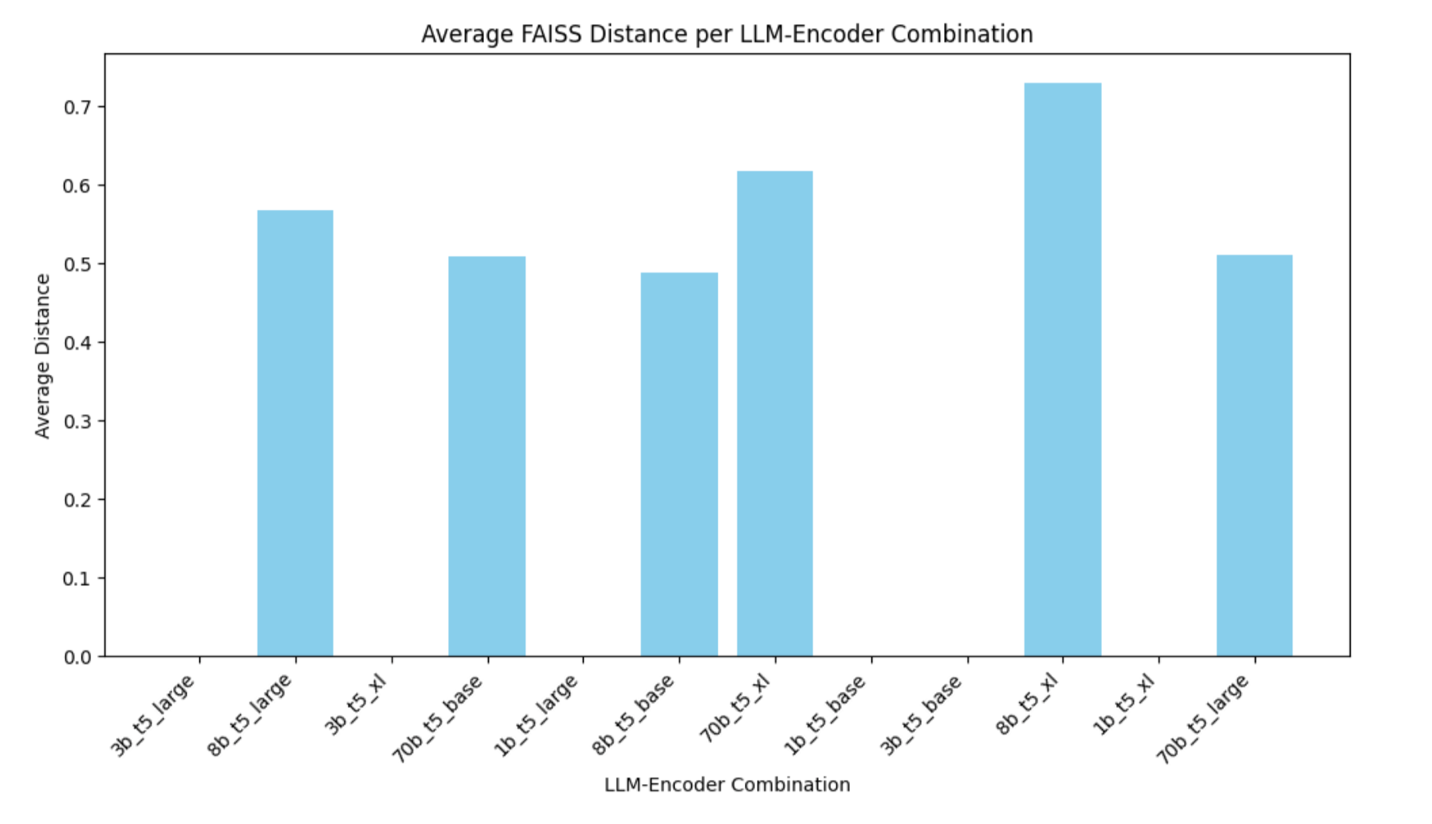
Figure : Average FAISS distance by model and encoder
The chart shows that the 1B and 3B models yield an average FAISS distance of zero, meaning their expanded‑interest embeddings are essentially identical and offer no differentiation. By contrast, the 8B model produces a distance of about 0.5 with t5‑base, rising further with t5‑large and t5‑xl, which demonstrates that larger encoders capture more of the model’s nuance. The 70B model only adds a small boost—and only with the XL encoder—so its extra cost yields limited benefit.
In practical terms, a Llama 8B LLM paired with a base or large T5 encoder delivers clear separation in embedding space without the higher inference time and resource usage of a 70B model.
Comparing model and encoder impact on embedding spread
To see how LLM size and encoder scale shape our embedding space, you can measure—for each LLM and encoder pair—the mean FAISS distance from a representative expanded interest vector to its top 10 neighbors. The following bar chart plots those averages side by side. You can instantly spot that 1B and 3B collapse to zero, 8B jumps to around 0.5 and rises with larger encoders, and 70B only adds a small extra spread at the XL scale. This helps you choose the smallest combination that still gives you the embedding diversity needed for effective cold‑start recommendations.
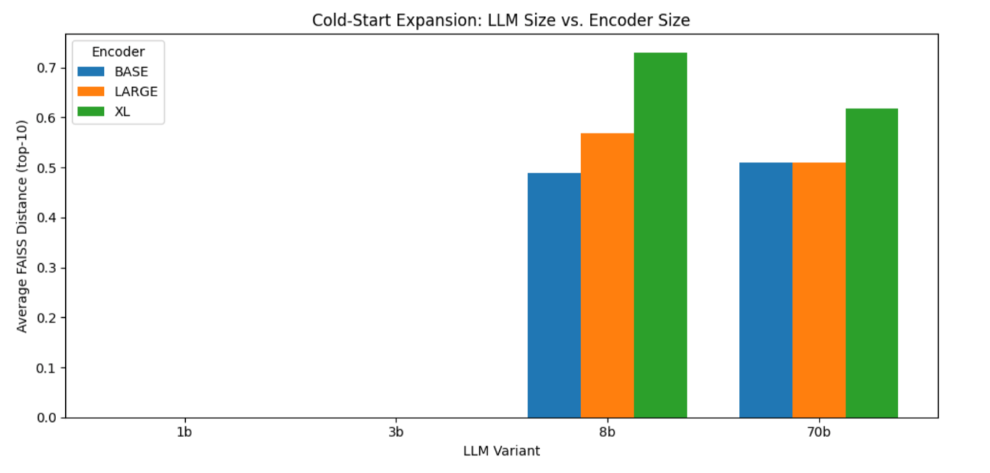
Figure : FAISS distance by LLM and encoder size
Evaluating recommendation overlap across Llama variations and encoders to balance consistency and novelty
In the next analysis, you build a basic recommend_books helper that, for various LLM sizes and encoder choices, loads the corresponding expanded‑interest DataFrame, reads its FAISS index, reconstructs the first embedding as a stand‑in query, and returns the top-k book titles. Using this helper, we first measure how much each pair of encoders agrees on recommendations for a single LLM—comparing base compared to large, base compared to XL, and large compared XL—and then, separately, how each pair of LLM sizes aligns for a fixed encoder. Finally, we focus on the 8B model (shown in the following figure) and plot a heatmap of its encoder overlaps, which shows that base and large share about 40% of their top 5 picks while XL diverges more—illustrating how changing the encoder shifts the balance between consistency and novelty in the recommendations.
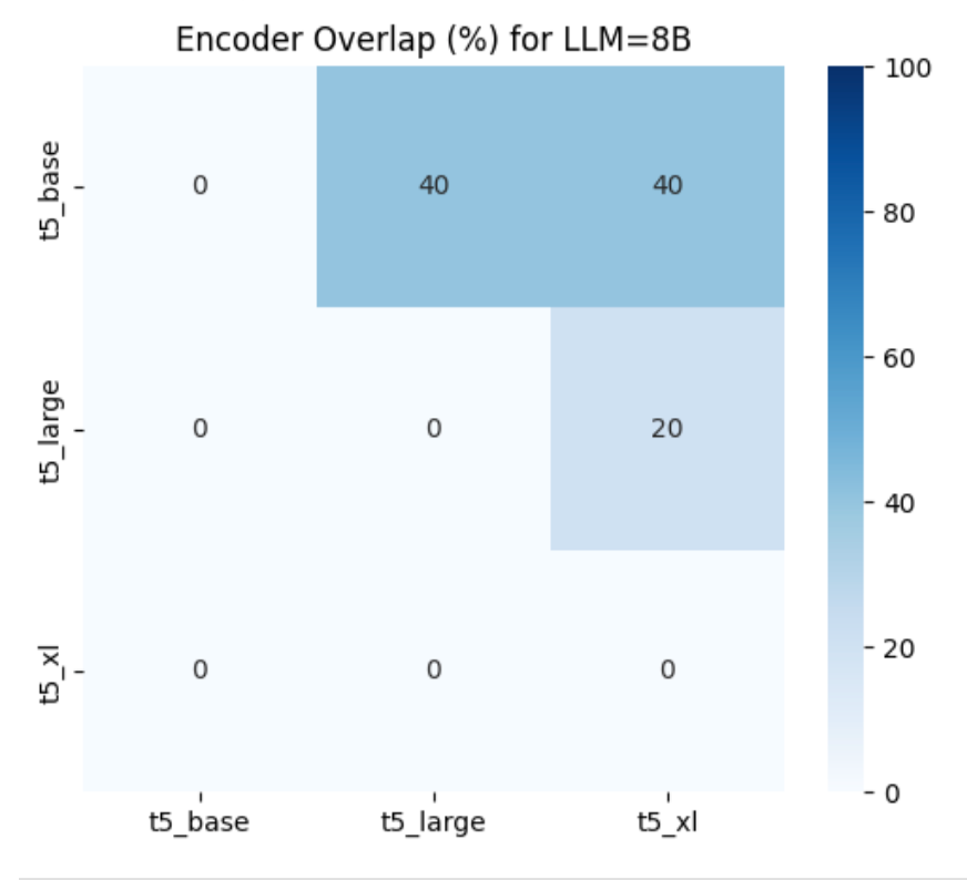
Figure : 8B model: encoder overlap heatmap
For the 8B model, the heatmap shows that t5_base and t5_large share 40% of their top 5 recommendations, t5_base and t5_xl also overlap 40%, while t5_large vs t5_xl overlap only 20%, indicating that the XL encoder introduces the greatest amount of novel titles compared to the other pairs.
Tweaking tensor_parallel_size for optimal cost performance
To balance inference speed against resource cost, we measured how increasing Neuron tensor parallelism affects latency when expanding user interests with the Llama 3.1 8B model on a trn1.32xlarge instance. We ran the same zero‑shot expansion workload at tensor_parallel_size values of 2, 8, 16, and 32. As shown in the first chart, P50 Latency falls by 74 %—from 2,480 ms at TP = 2 to 650 ms at TP = 16—then inches lower to 532 ms at TP = 32 (an additional 18 % drop). The following cost-to-performance chart shows that beyond TP = 16, doubling parallelism roughly doubles cost for only a 17 % further latency gain.
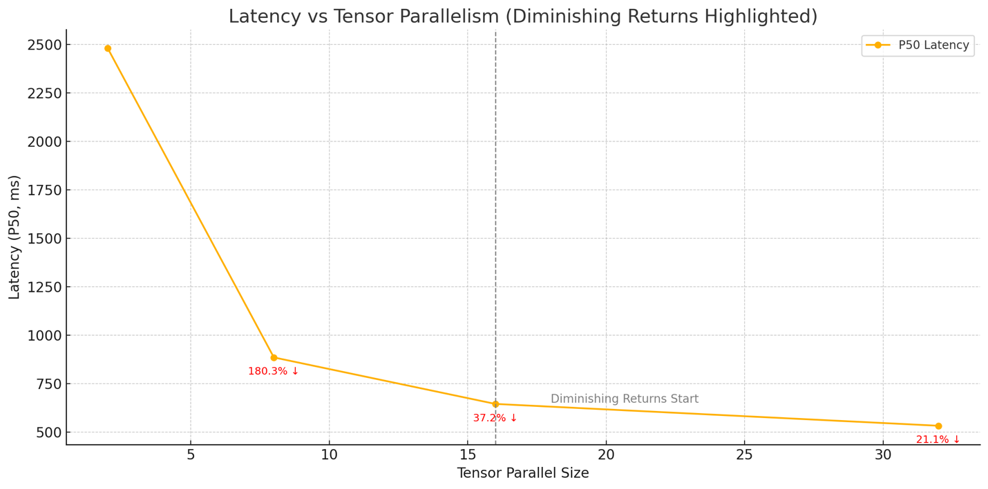
Figure : Latency compared to tensor parallel size
In practice, setting tensor_parallel_size to 16 delivers the best trade‑off: you capture most of the speed‑up from model sharding while avoiding the sharply diminishing returns and higher core‑hour costs that come with maximal parallelism, as shown in the following figure.
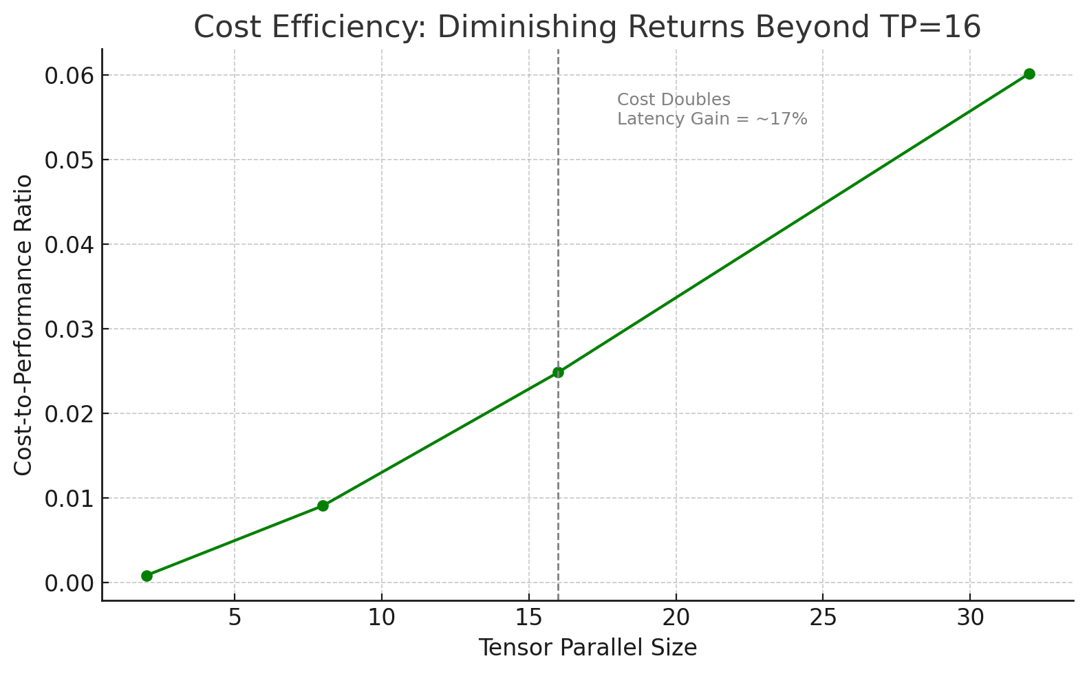
Figure : Cost-performance compared to tensor parallel size
The preceding figure visualizes the cost-to-performance ratio of the Llama 8B tests, emphasizing that TP=16 offers the most balanced efficiency before the benefits plateau.
What’s next?
Now that we have determined the models and encoders to use, as well as the optimal configuration to use with our dataset, such as sequence size and batch size, the next step is to deploy the models and define a production workflow that generates expanded interest that is encoded and ready for match with more content.
Conclusion
This post showed how AWS Trainium, the Neuron SDK, and scalable LLM inference can tackle cold-start challenges by enriching sparse user profiles for better recommendations from day one.
Importantly, our experiments highlight that larger models and encoders don’t always mean better outcomes. While they can produce richer signals, the gains often don’t justify the added cost. You might find that an 8B LLM with a T5-large encoder strikes the best balance between performance and efficiency.
Rather than assuming bigger is better, this approach helps teams identify the optimal model-encoder pair—delivering high-quality recommendations with cost-effective infrastructure.
About the authors
 Yahav Biran is a Principal Architect at AWS, focusing on large-scale AI workloads. He contributes to open-source projects and publishes in AWS blogs and academic journals, including the AWS compute and AI blogs and the Journal of Systems Engineering. He frequently delivers technical presentations and collaborates with customers to design Cloud applications. Yahav holds a Ph.D. in Systems Engineering from Colorado State University.
 Nir Ozeri Nir is a Sr. Solutions Architect Manager with Amazon Web Services, based out of New York City. Nir leads a team of Solution Architects focused on ISV customers. Nir specializes in application modernization, application and product delivery, and scalable application architecture.
