Published on July 22, 2025 8:36 PM GMT

Repo: https://github.com/DavidUdell/sparse_circuit_discovery

TL;DR: A SPAR project from a while back. A replication of an unsupervised circuit discovery algorithm in GPT-2-small, with a negative result.

Thanks to Justis Mills for draft feedback and to Neuronpedia for interpretability data.

Introduction

I (David) first heard about sparse autoencoders at a Bay Area party. I had been talking about how activation additions give us a map from expressions in natural language over to model activations. I said that what I really wanted, though, was the inverse map: the map going from activation vectors over to their natural language content. And, apparently, here it was: sparse autoencoders!

The field of mechanistic interpretability quickly became confident that sparse autoencoder features were the right ontology for understanding model internals. At the high point of the hype, you may recall, Anthropic declared that interpretability had been reduced to "an engineering problem."

Frustratingly, though, the only naturalistic model behavior that had been concretely explained at that point was indirect object identification, dating from back before the sparse autoencoder revolution! In a world where sparse autoencoders just solved it, I would expect everyone and their dog to be sharing pseudocode fully explaining pieces of LLM behavior. On the sparse autoencoder circuits front, here was a representative proffered explanatory circuit at that time:

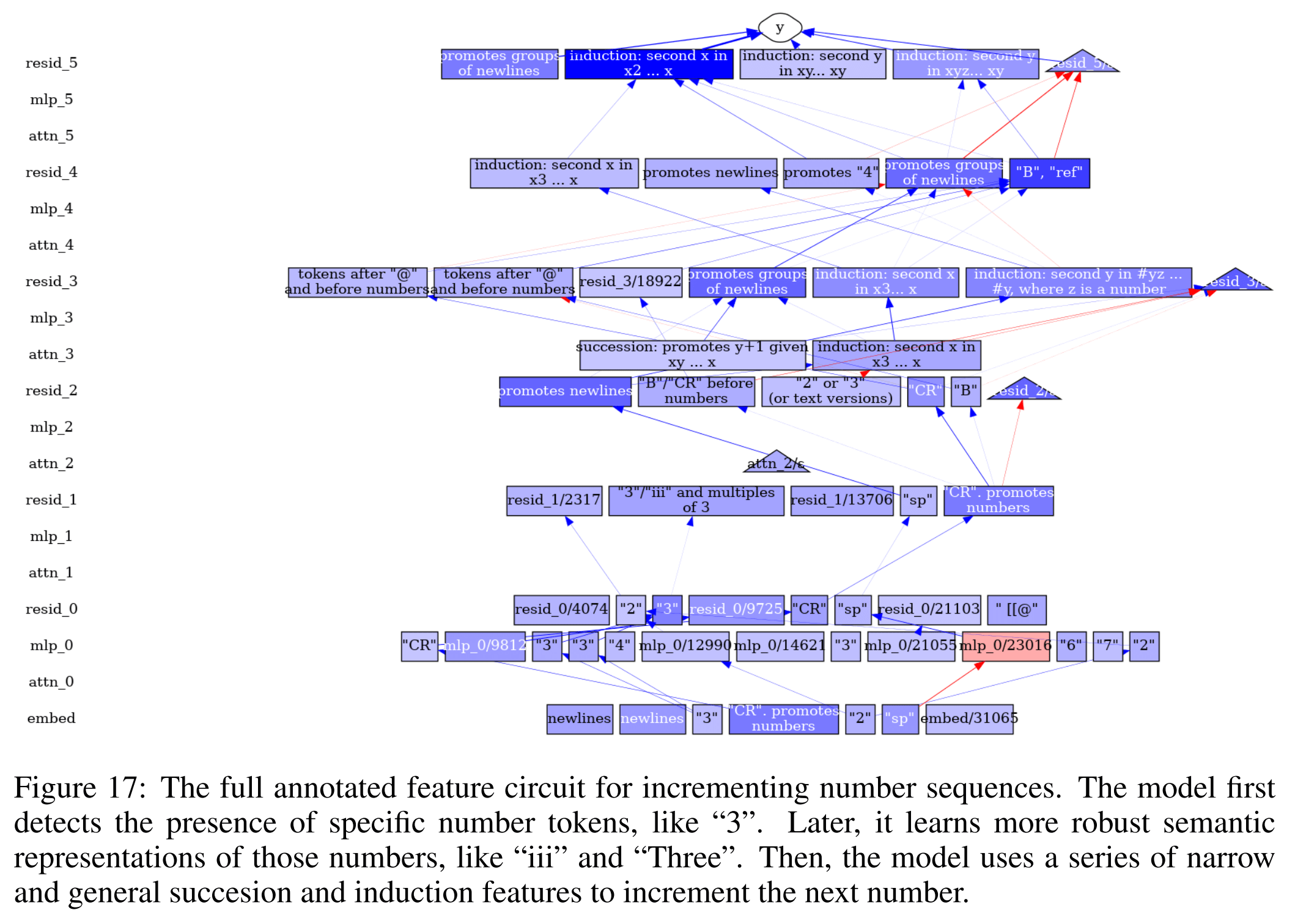
I cannot directly interpret this image as pseudocode, is the thing. Note that it's definitely true that the features highlighted here are often quite *relevant* and *suggestive*. But the *edges* between features don't really add to my understanding of what is going on. I get the feeling that the crisp mechanistic understanding is *tantalizingly close* here... but still out of reach.

So it struck me as strange that so much capital was being put into tweaking and refining the sparse autoencoder architecture, and not into leveraging existing autoencoders to explain stuff—I thought the whole point was that we had the right ontology for explanations already in our hands! Maybe not full explanations of every model behavior, but full explanations of some model behaviors nonetheless.

The theory of change that this then prompted for our SPAR project was: show how any naturalistic transformer behavior can be concretely explained with sparse autoencoder circuit discovery. Alternatively, show how concrete sparse autoencoder circuits fail as full explanations. So that's what we did here: we replicated the then-new circuit discovery algorithm, ironed out a few bugs, and then tried to mechanistically explain how some GPT-2 forward passes worked. It did not work out, in the end.

Our bottom-line conclusion, driven by our datapoint, is that the localistic approximations of vanilla sparse autoencoders cannot be strung together into fully explanatory circuits. Rather, more global, layer-crossing approximations of the model's internals are probably what is needed to get working explanatory circuits.

Gradient-Based Unsupervised Circuit Discovery

An explanation of the circuit discovery algorithm from Marks et al. (2024) that we replicate.

We want to be able to explain a model's behavior in any arbitrary forward pass by highlighting something in its internals. Concretely, we want to pinpoint a circuit that was responsible for that output in that context. That circuit will be a set of sparse autoencoder features and their causal relations, leading to the logit for the token being upweighted and other-token logits being downweighted.

The most basic idea for capturing causality in mechanistic interpretability is: take derivatives. If you want to know how a scalar $x$ affected a scalar $y$ , well, take the derivative of $y$ with respect to $x$ . If you want to know how anything affected the loss, of course, take the derivative of the loss with respect to it. But the strategy is fully general: if you want to know how one activation affected another activation, take the derivative of the one with respect to the other. And if you want to know how your sparse autoencoder features all affect one another, just take derivatives among them.

The idea of the sparse autoencoders themselves is less immediately obvious. Once you have them, though, they are a differentiable quantity that automatically lend themselves to causal approximation. A natural next step after you get apparently comprehensible sparse autoencoder features is to see whether their causal relationships match (or fail to match) your understanding of feature contents.

On the implementation side, derivatives batch well in PyTorch. In a small number of backward passes, we can estimate how sparse autoencoder features causally interrelate.

More precisely, let $L$ be the loss (concretely: CrossEntropy). Let $f$ be a sparse-autoencoder feature activation, a scalar, with a suppressed index for its model sublayer $i$ :

f \in \to f \in R^{d_{a u t o e n c o d e r}}

A node $n_{f}$ for a feature $f$ is given by

f \cdot \frac{\partial L}{\partial f}

Interpret a node as a feature's individual contribution to the loss.

An edge between two feature activations $f_{i}$ and $f_{j}$ is given by

f_{i} \cdot \frac{\partial f_{j}}{\partial n_{f_{i}}}

Interpret an edge as the $i$ feature's individual contribution to the loss by way of affecting the $j$ feature.

Collect the absolutely largest nodes at every sublayer $i$ in a forward pass. Compute the edges between all neighboring nodes in the collection. Finally, correct for any double-counted causal effects between the nodes.^[1]

The graph of edges you have now (or, precisely, the subset of that graph that paths to the logits) is a gradient approximation of the actual causal relationships between sparse autoencoder features. It is, putatively, an explanation of that forward pass.

Sanity Check

A spot check of the new method's validity.

Last time, we looked at the prompt Copyright (C). GPT-2-small knows that that final closing parenthesis should be coming: the model puts the majority of its probability on that token. How does it know to do that?

Well, last time, we saw persistent "causal threads" in GPT-2-small's residual stream over that forward pass. Certain sparse autoencoder features can be seen causally propagating themselves across a forward pass, just preserving their own meaning for later layers. The features that we observe doing this specifically look like hypotheses about what that model's next token will be. For example, for the Copyright (C prompt there are a couple of causal threads about word completions for the capital letter C. There is a causal thread for tracking that you're inside an open parenthetical, and one for acronym completions.

Run that same forward pass through this new gradient-based method, using the old residual autoencoders only. This method also picks out at least one of those same causal threads—a C-words one—as its top highlight.

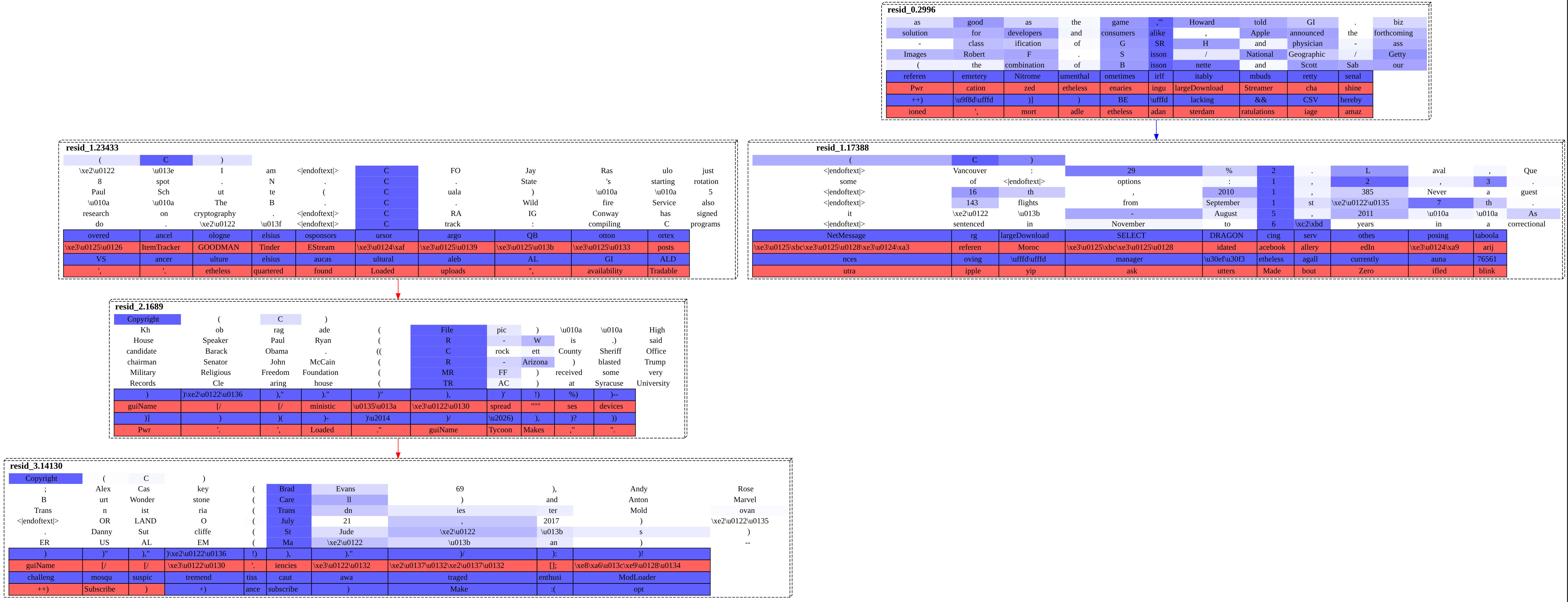
The graph is definitely hard to read. Just round it off to: we're passing this sanity check, as we're at least recovering a common structure with both methods.

Results

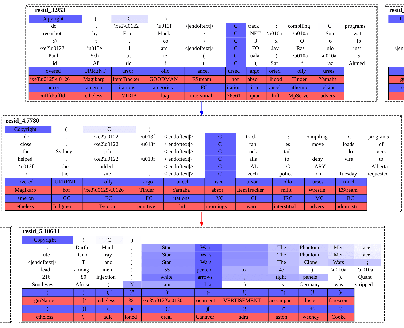
Okay, here's our argument against the gradient-based method. If a circuit is explanatory, when you walk back through its graph, each node and edge adds to the story. In particular, the very final nodes should be explanatory; if they aren't, that screens off the rest of the graph being explanatory.

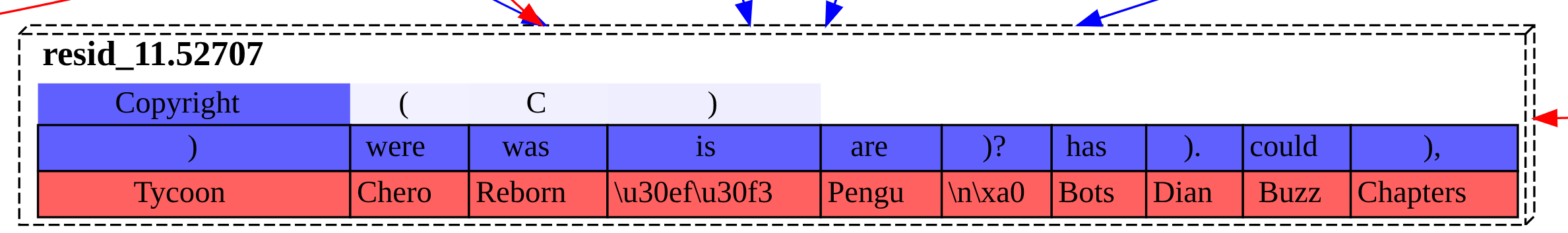
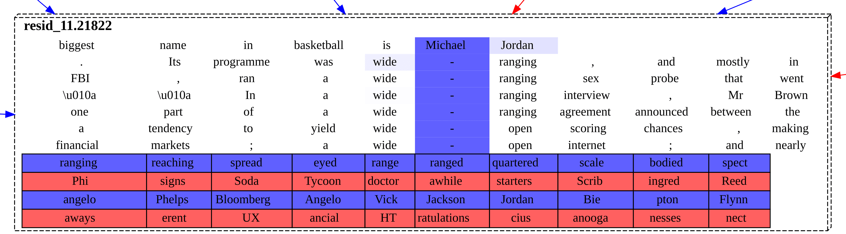
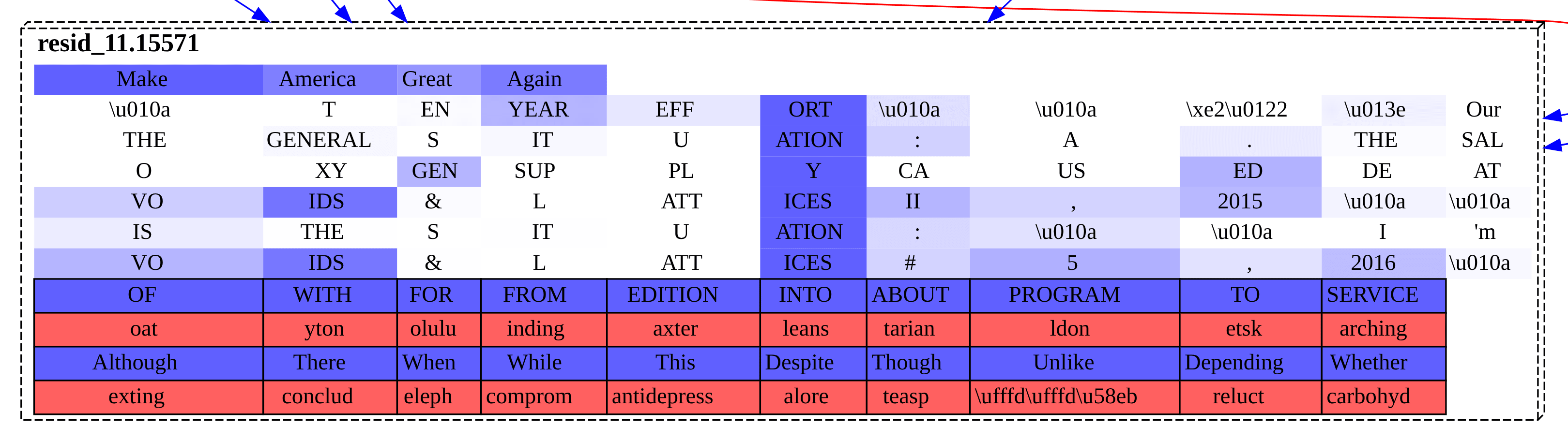
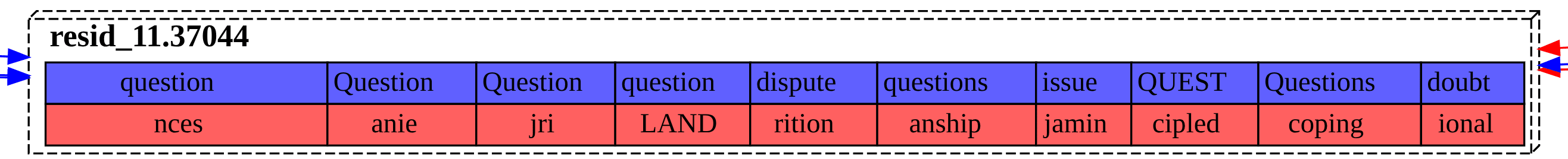
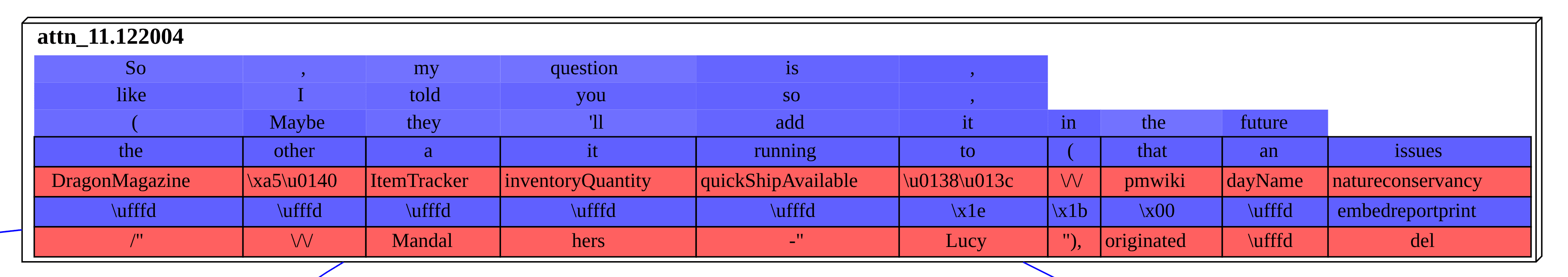
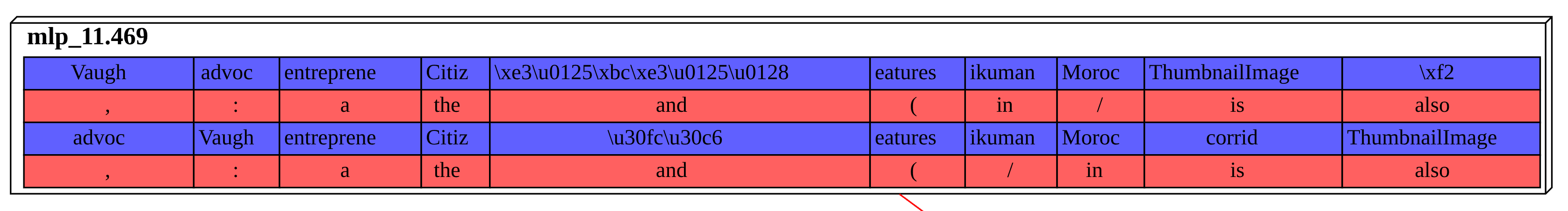
Below are the single top feature nodes for the token following each prompt. These nodes are then the main interpretable proximal cause for the model's logits, according to this sparse autoencoder circuit discovery framework. We are interpreting each node using its bottom-most blue row of boxes. That blue row represents the tokens that were most promoted by the feature in its forward pass. (Importantly, it is causal, not correlational, interpretability data.) Focus on that bottom-most blue row of logit boxes promoted.^[2]

Top Proximal Causes

1. `Copyright (C`

Top Completions
Token	Probability
`)`	82%
`VS`	1%
`AL`	1%
`IR`	0%
`)(`	0%

2. `The biggest name in basketball is Michael`

Top Completions
Token	Probability
`Jordan`	81%
`Carter`	4%
`Kidd`	3%
`Be`	2%
`Malone`	1%

3. `Make America Great`

Top Completions
Token	Probability
`Again`	95%
`again`	3%
`"`	0%
`Again`	0%
`."`	0%

4. `To be or not to be, that is the`

Top Completions
Token	Probability
`question`	6%
`way`	5%
`only`	3%
`nature`	3%
`point`	2%

5. `Good morning starshine, the Earth says`

Top Completions
Token	Probability
`hello`	9%
`it`	7%
`,`	6%
`:`	4%
`that`	4%

Causal Structure From All Sublayers

Of those five examples, only two seem to correctly call the model's top next token: the closing parentheses feature and the question feature. But, even when you condition on having an actually predictive proximal feature, the sublayer upstream edges and nodes flowing into it—plotting whose contributions is the whole point of this—are not illuminating.

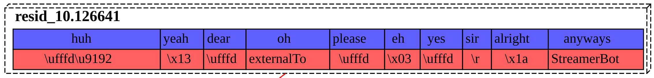
The edges from each upstream sublayer that most strongly affected the closing parentheses feature were:

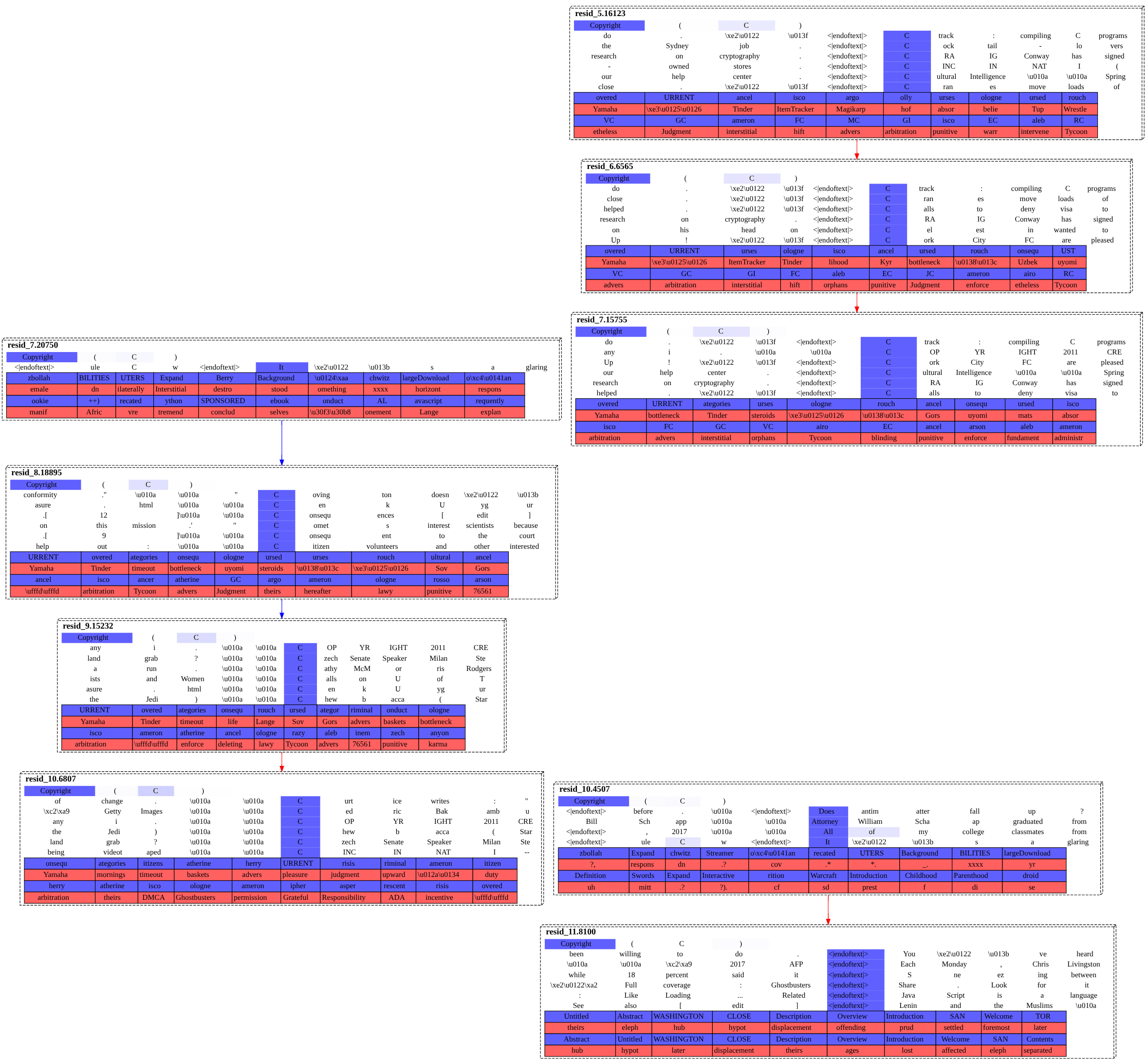
The edges from each upstream sublayer that most strongly affected the question feature were:

Casual exclamations; same node as before

When you ablate out a causal thread with a clear natural interpretation to it, the logit effects seem quite sensible.^[3] Also, you can often scan over a causal graph that you get out of this method and cherry-pick a sensible, informative node activation: you can learn, e.g., that a particular attention layer seems to have been particularly counterfactual for that token.

Our complaint is that you are really not getting mechanistic understanding of the reasons why the model is writing what it is into the residual stream. It was that "reasons why" that we were after here in the first place.

Conclusion

We went into this project hoping to plug a research gap, and get out a concrete algorithmic explanation of what is going on in a naturalistic forward pass, given autoencoder features are taken to be primitives. We found that that didn't work with this algorithm.

Relatively recently, Anthropic published work showing cross-layer transcoder circuit discovery that does work to that standard. They give the full cognitive algorithm that Claude is using for two-digit addition, e.g. Their result leads us to think that it is the "cross-layer-ness" of what they were doing that is really the special sauce there. If the autoencoder circuits we played with here are built out of local approximations to what the model is representing at various points in the forward pass, cross-layer transcoders are instead built out of global approximations. Our overall update is that the additional work of getting that global approximation is necessary to make circuits research work in naturalistic transformers.

^{^}
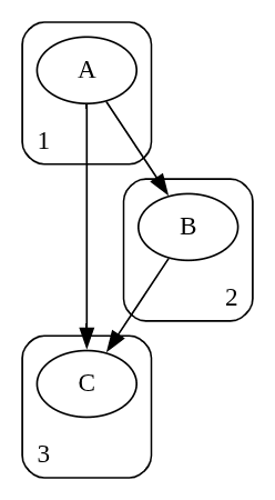
Say that you have three nodes, $A$ , $B$ , and $C$ , at model sublayers $1$ , $2$ , and $3$ , respectively. Because of the residual stream, model topology is such that, in a forward pass, causality goes as follows
If you want the value of the edge $A \to C$ , you cannot just compute the effect of node $A$ on node $C$ . You will also have to subtract off any effect due to the confounding path $A \to B \to C$ .
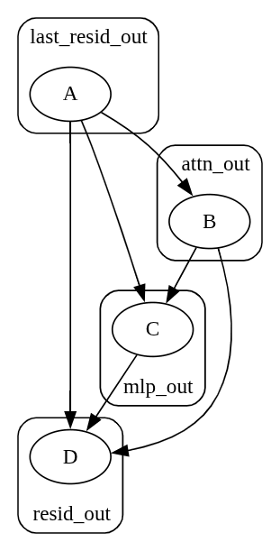
Say you now have four nodes, $A$ , $B$ , $C$ , and $D$ , at model sublayers last_resid_out, attn_out, mlp_out, and resid_out, respectively. Causality here goes
The edges $A \to B$ , $B \to C$ , and $C \to D$ can be simply computed without any needed corrections.
The edge $A \to C$ has the confounding path $A \to B \to C$ .
The edge $B \to D$ has the confounding path $B \to C \to D$ .
The edge $A \to D$ has the confounding paths $A \to B \to D$ , $A \to C \to D$ , and $A \to B \to C \to D$ .
^{^}
The topmost piece of interpretability data is a set of sequences for which the feature most activated, shaded accordingly. It is correlational data.
Red rows of logit boxes are just the opposite of the blue rows: they are the logits that are causally most suppressed by the feature.
The reason that there are sometimes multiple blue (and red) rows in a cell is that the rows are sourced from both local data and, when available, from Neuronpedia. The reason to focus on the bottom-most blue row is that that is the local data row, giving the causal effects of that feature for this particular forward pass.
^{^}
This wasn't done suitably at scale last time, but validation results (ablation over a significant dataset subset) do clean up at scale.

Discuss

Introduction

Gradient-Based Unsupervised Circuit Discovery

Sanity Check

Results