本文深入探讨了稀疏自编码器（SAE）中L0（平均激活的隐变量数量）这一设计选择对特征学习的关键影响。研究发现，当SAE的L0低于底层特征的真实L0时，SAE会通过“作弊”学习到错误的特征混合，从而获得更低的均方误差（MSE）损失，尤其对高频特征影响更为严重。反之，若SAE的L0高于真实L0，则会出现退化解但不会进行特征对冲。文章通过一个带有相关特征的玩具模型实验，展示了不同L0设置下的具体表现，并提出通过混合低L0和高L0的损失项，可能实现对真实特征的有效学习，这为解决“真实L0未知”的问题提供了新的思路，强调L0不应是随意设置的超参数，而应是需要被发现的目标。

🎯 **L0过低导致特征对冲与错误学习**：当SAE的L0设置低于数据底层特征的真实激活数量时，SAE为了优化MSE损失，会采取“特征对冲”策略，即通过混合（合并）相关特征来避免单独表示某个特征，导致学习到的特征不准确。这种现象在高频特征上表现得尤为明显，因为它们需要更精细的表示，但受限于较低的L0，SAE会“作弊”以获得更好的MSE表现，尽管这牺牲了特征的准确性。

📈 **L0过高导致退化解但无特征对冲**：若SAE的L0设置高于底层特征的真实激活数量，模型虽然可能学习到一些不完美的、退化的解决方案，但不会出现特征对冲的行为。这意味着模型不会系统性地混合或扭曲特征，而是可能存在多个同样能达到低损失的解决方案，但由于没有明确的“正确”L0指导，模型倾向于选择其中一个非最优的表示。随着L0的增加，退化情况会更加严重。

🔄 **混合L0损失实现鲁棒特征学习**：研究表明，通过在训练过程中同时引入一个较低的L0损失和一个较高的L0损失，可以有效缓解L0设置不当带来的问题。低L0损失能够约束高L0损失避免学习退化解，而高L0损失则能防止低L0损失陷入特征对冲。这种“多L0”的训练方式，类似于Matryoshka SAEs的思路，为在未知真实L0的情况下学习到准确的底层特征提供了一种可行的方法。

💡 **L0应被视为待发现的目标而非随意超参数**：文章的核心观点之一是，L0不应被视为一个可以随意调整的超参数。相反，它应该被看作是数据内在属性的一部分，存在一个“正确”的L0值，能够最有效地表示底层特征。研究结果表明，选择错误的L0会导致显著的性能下降，因此，未来的工作应专注于如何识别和利用数据的真实L0，以训练出更准确、更鲁棒的SAE模型。

Published on July 19, 2025 1:51 PM GMT

When we train Sparse Autoencoders (SAEs), the sparsity of the SAE, called L0 (the number of latents that fire on average), is treated as an arbitrary design choice. All SAE architectures include plots of L0 vs reconstruction, as if any choice of L0 is equally valid. 

However, recent work that goes beyond just calculating sparsity vs reconstruction curves shows the same trend: low L0 SAEs learn the wrong features ^[1][2]. 

In this post, we investigate this phenomenon in a toy model with correlated features and show the following:

If the L0 of the SAE is lower than the true L0 of the underlying features, the SAE will "cheat" to get a better MSE loss score than a correct SAE would achieve by learning broken mixtures of correlated features. This can be viewed as a form of feature hedging^[3]. This is worse the lower the L0 of the SAE, and affects high-frequency features more severely.If the L0 of the SAE is higher than the true L0 of the underlying features, the SAE will find degenerate solutions, but does not engage in feature hedging. This is worse the higher the L0 of the SAE.If we mix together a too-low L0 loss with a too-high-L0 loss, we can learn the true features (like a Matryoshka SAE^[2], except with multiple L0s instead of multiple widths). This may provide a way to learn a correct SAE despite not knowing the "true L0" of the underlying training data.

The phenomenon of poor performance due to incorrect L0 can be viewed from the same lens of Feature Hedging: If we do not give SAEs enough resources in terms of L0 or width to reconstruct the input, the SAE will find ways to cheat by learning incorrect features. In light of this, we feel that L0 should not be viewed as an arbitrary hyperparameter. We should assume that there is a "correct" L0, and we should aim to find it.

In the remainder of this post, we will walk through our experiments and results. Code is available in this Colab Notebook.

Toy model setup

We set up a toy model with 20 mutually-orthogonal true features $f_0$ through $f_{19}$,  where features 1-19 are positively correlated with $f_0$. For each of these features, we assign a base firing probability $P_i$. Feature $f_i$ fires with probability $P_i$ if feature 0 is firing, and probability $0.5\ast P_i$ if $f_0$ is not firing. Thus, each feature can fire on its own, but is more likely to fire if $f_0$ is also firing. Feature $f_0$ fires with probability $0.35$, and $P_1$ through $P_{19}$  linearly decreases from $0.74$ to $0.19$, so that $f_0$ is more likely to fire overall than $f_1$, and $f_1$ is more likely to fire than $f_2$, etc... To keep everything simple, each feature fires with mean magnitude $1.0$ and stddev $0.15$. The stddev is needed to keep the SAE for engaging in Feature Absorption^[4], as studying absorption is not the goal of this exploration.

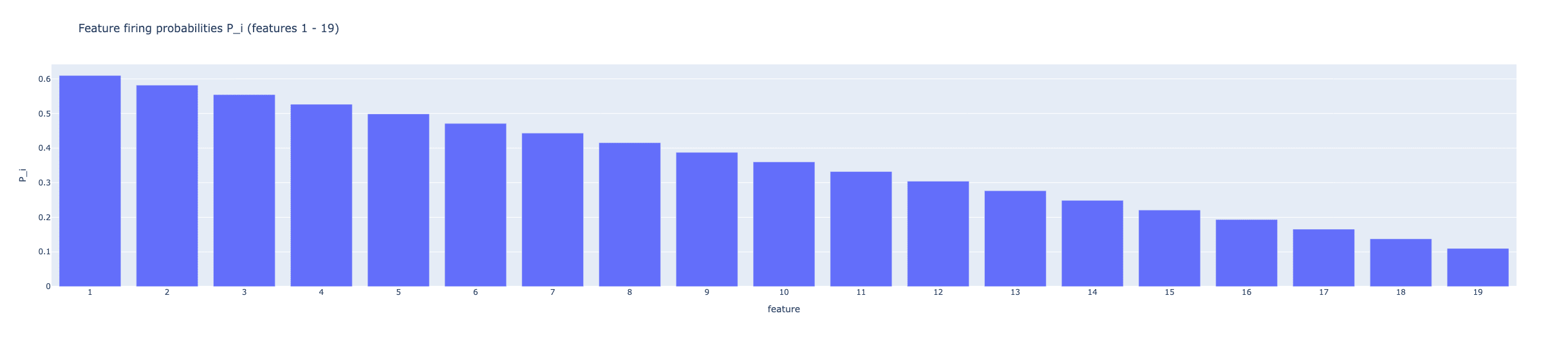
These probabilities were chosen so the true L0 (the average number of features active per sample) is roughly 5.

SAE setup

We use a Global BatchTopK SAE^[5] with the same number of latents (20) as the number of features in our toy model. We use a BatchTopK SAE to allow us to control the L0 of the SAE directly so we can study the effect of L0 in isolation of everything else. The SAE is trained on 25 Million samples generated from the toy model.

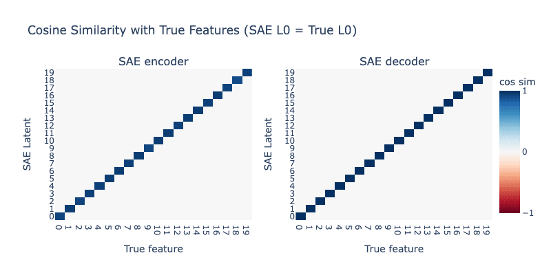
Case 1: SAE L0 = Toy Model L0

We begin by setting the L0 of the SAE to 5 to match the L0 of the underlying toy model. As we would hope, the SAE perfectly learns the true features.

 Case 2: SAE L0 < Toy Model L0

Next, we set the L0 of the SAE to 4, just below the correct L0 of 5. The results are shown below:

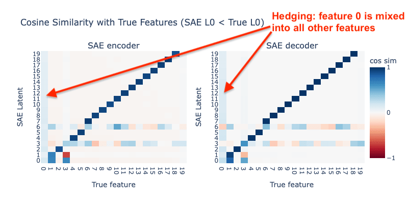
We now see clear signs of hedging: the SAE has decided to mix $f_0$ into all other latents to avoid needing to represent it in its own latent. In addition, the latents tracking high-frequency features (features 1-5) appear much more broken than latents tracking lower-frequency latents.

Cheating improves MSE loss

Why would the SAE do this? Why not still learn the correct latents, and just fire 4 of them instead of 5? Below, we calculate the mean MSE loss from using the correct SAE from Case 1, except selecting the top 4 instead of 5 features, with the broken SAE we trained in Case 2.

	MSE loss
Case 1 (correct) SAE, trained with k=5 and cut to k=4	0.53
Case 2 (broken) SAE, trained with k=4	0.42

Sadly, the broken behavior we see above achieves better MSE loss than correctly learning the underlying features. We are actively incentivizing the SAE to engage in feature hedging and learn broken latents when the SAE L0 is too low.

Lowering SAE L0 even more

Next, we lower the L0 of the SAE further, to 3. Results are shown below:

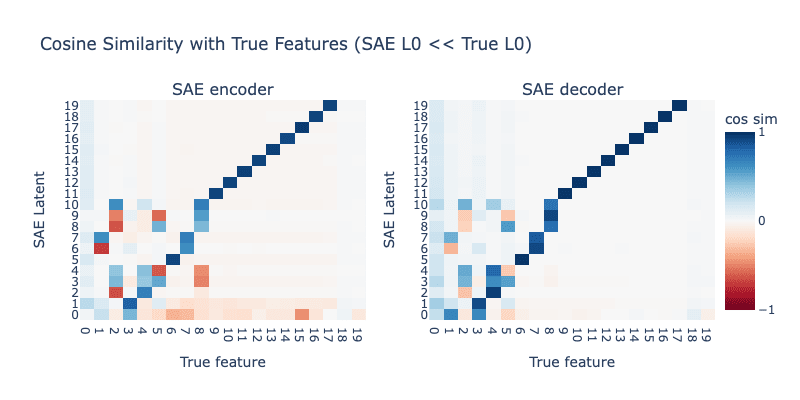
Lowering L0 further to 3 makes everything far worse. Although it's hard to tell from the plot, the magnitude of hedging (the extent to which $f_0$ is mixed into all other latents) is higher than with L0=4, and now all latents tracking higher-frequency features (features 1-10) are completely broken.

Case 3: SAE L0 > Toy Model L0

What happens if we set the SAE L0 too high? We now set the L0 of the SAE to 6. Results are shown below:

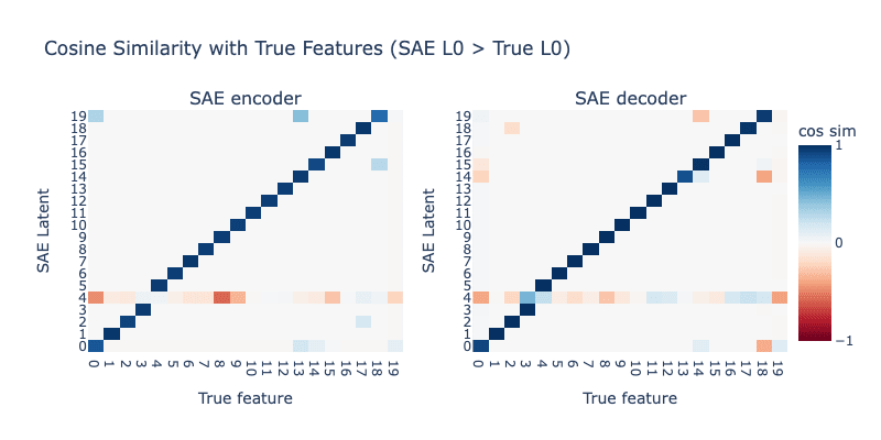
We see that the SAE learns some slightly broken latents, but there is no sign of systematic hedging. Instead, it seems like having too high of a L0 makes it so there are multiple ways to get perfect reconstruction loss, so we should not be surprised that the SAE settles into an imperfect result.

Increasing L0 even more

Next, we see what happens when we increase the SAE L0 even further. We set SAE L0 to 8. Results are shown below:

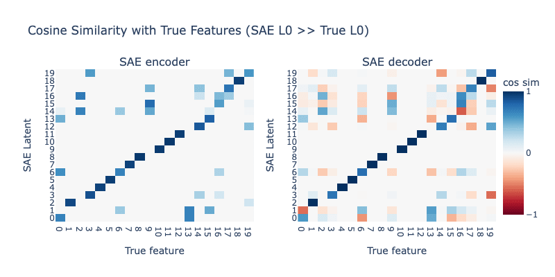
We now see the SAE is learning far worse latents than before, with most latents being completely broken. However, we still don't see any sign of systematic hedging like we saw with low L0 SAEs.

Mixing high and low L0 penalties together

Clearly, if we knew the correct L0 of the underlying data, the best thing to do is to train at that L0. In reality, we do not yet have a way to find the true L0, but we find that we can still improve things by mixing together two MSE losses during training: One loss uses a low L0 and another uses a high L0.

This is conceptually similar to how Matryoshka SAEs^[3] work. In a Matryoshka SAE, multiple losses are summed using different width prefixes. Here, we sum two losses using different L0s:

$$L=L_{k_1}+\lambda L_{k_2}$$

In this formualtion, $L_{k_1}$ is the MSE loss term using a lower L0, and $L_{k_2}$ is the MSE loss term using a higher L0. We add a coefficient $\lambda$ so we can control the relative balance of these two losses.

Below, we train an SAE with $k_1=4$, $k_2=8$, $\lambda =1$:

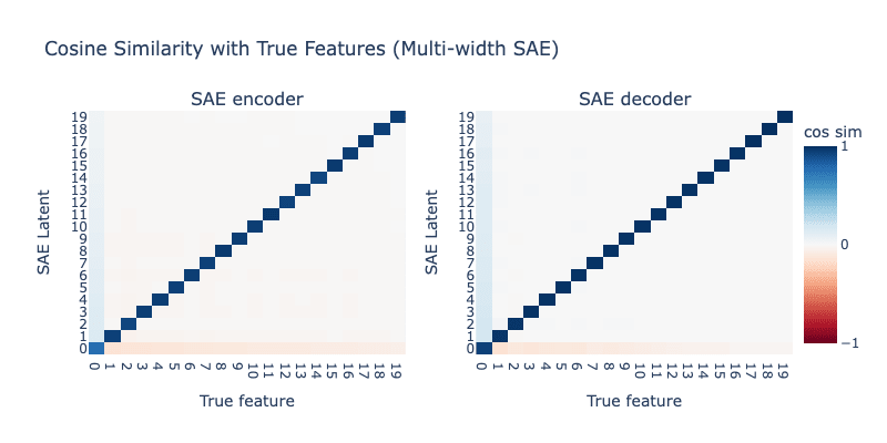
This looks a lot better than our Case 1 SAE - we still see a dedicated latent for $f_0$, but there's also clear hedging going on still. Let's try increasing $\lambda$ further to 20:

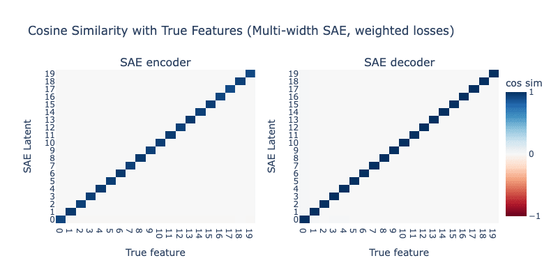
We've now perfectly recovered the true features again! It seems like the low-L0 loss helps keep the high-L0 loss from learning a degenerate solution, while the high-L0 loss keeps the low-L0 loss from engaging in hedging.

 

1. ^{^}

   Kantamneni, Subhash, et al. "Are Sparse Autoencoders Useful? A Case Study in Sparse Probing." Forty-second International Conference on Machine Learning.

2. ^{^}

   Bussmann, Bart, et al. "Learning Multi-Level Features with Matryoshka Sparse Autoencoders." Forty-second International Conference on Machine Learning.

3. ^{^}

   Chanin, David, Tomáš Dulka, and Adrià Garriga-Alonso. "Feature Hedging: Correlated Features Break Narrow Sparse Autoencoders." arXiv preprint arXiv:2505.11756 (2025).

4. ^{^}

   Chanin, David, et al. "A is for absorption: Studying feature splitting and absorption in sparse autoencoders." arXiv preprint arXiv:2409.14507 (2024).

5. ^{^}

   Bussmann, Bart, Patrick Leask, and Neel Nanda. "BatchTopK Sparse Autoencoders." NeurIPS 2024 Workshop on Scientific Methods for Understanding Deep Learning.

Discuss