
Published on July 11, 2025 4:06 PM GMT
This post contains a summary of our paper which will be presented at ICML 2025. Feel free to visit me (Lukas) at our poster stand to chat about our work. More info about the time and location can be found here.
TL;DR
Reward learning techniques like RLHF are still the go-to method to align current state-of-the-art large language models (LLM). However, these techniques are by no means perfect. In particular, the discovery of jailbreaks and related issues shows that correctly aligning LLMs to human values remains a hard-to-solve problem.
Motivated by these issues, we perform a mathematical analysis of reward learning techniques, and focus on figuring out when a data distribution used to train a reward model will produce a reward model whose optimal policy has provably low regret.
Our analysis shows that for many reward learning techniques large classes of realistic data distributions are not worst-case safe, thereby providing a potential explanation for the observed shortcomings of current reward learning techniques such as RLHF.
Epistemic Status: Our paper does a worst-case analysis for the regret of a policy when a reward model is learned up to a given loss. Deep learning is known for performing better than the worst-case in many settings, and so this should also hold for reward learning when built upon deep learning. It remains to be determined to what extent the worst-case failures we analyze here are the source of errors observed in practice in methods like RLHF.
Acknowledgements: Thanks a lot to Leon Lang, Alessandro Abate, Patrick Forré, David Krueger, and Joar Skalse, all co-authors of the paper. Special thanks to Leon Lang, who developed many of the core results and provided useful feedback on the draft of this post, and Joar Skalse, who developed the project idea and provided close supervision during the project’s duration.
Introduction
Reward learning has become a useful tool to train AI systems with reinforcement learning (RL), especially for tasks where specifying a reward function manually is challenging. The basic idea of reward learning is to learn the reward function from data instead of specifying it manually. Learning a reward model enabled the development of powerful reinforcement learning techniques, such as reinforcement learning from human feedback (RHLF) which has become the de facto standard for aligning pretrained large language models (LLMs) to human values.
However, despite its widespread use and arguably good performance, techniques like RLHF are by no means perfect. In particular, the discovery of jailbreaks and related issues showed that correctly aligning LLMs to human values remains a hard-to-solve problem.
Motivated by these issues, we approach the problem of reward learning from a mathematical angle, and investigate under which conditions we can guarantee that reinforcement learning with reward learning does lead to a human-aligned policy. By abstracting over the specific reward-learning and policy optimization techniques, we are able to state general results that hold for many classes of reward-learning- and policy optimization algorithms. Our results show that achieving a worst-case safety guarantee is impossible for many (if not most) reasonable safety settings, providing a potential explanation for the existence of hard-to-fix error modes like jailbreaks.
Our results should be taken as weak evidence that basic techniques for aligning AI systems are not yet mature enough to be used to align AI systems that will be deployed in high-stakes settings. We claim that the deployment of such systems in settings where real harm can be caused necessitates some minimal guarantees about their safety.
Reward learning and its problems
A classical reward learning + RL pipeline consists of the following two main steps:
- First, a model of the reward function is learned from a dataset. It is assumed that this dataset is sampled from some underlying data distribution . The reward model is trained until it reaches a state of "convergence", after which the expected error on the training distribution usually is low.Second, a policy is trained using reinforcement learning techniques to optimize the learned reward model . The goal is for the policy to maximize the returns provided by the model that was learned in step 1.
While this setup has found widespread application, there also exist many criticisms of this framework. A non-exhaustive list of such problems include:
- Do humans even have a reward function?How do we aggregate the "reward functions" of different humans into a single reward function?Does the reward function of humans remain stable over time or change? What types of change do we want to allow?Partial observability of human feedback may lead to deceptionHumans might not reliably be able to supervise increasingly complex tasksHumans are irrational / their feedback is not Boltzmann rational, even when they oversee everything and the task is easy enough.
In this work, we ignore these problems and instead analyze reward learning from an optimization angle. In particular, we ask the following question:
Can reward learning guarantee low policy regret?
For any learning algorithm, it is a crucial question to know whether that algorithm is guaranteed to converge to a satisfactory solution. For example, in supervised learning for classification tasks, it can be shown that a learning algorithm producing a model with low empirical error (i.e., training error) is likely to achieve a low expected error (i.e., test error). The only requirements for this are sufficient training data and assuming that both the training and test data are drawn independently and identically distributed (i.i.d.) from a single stationary distribution.
However, reward learning differs from standard supervised learning in several key aspects. While a reward model with low training error is accurate relative to the training distribution, optimizing a policy to maximize the reward model can lead to a distributional shift. This occurs because the policy may explore regions of the data space that have very low probability under the training distribution. In these regions, the learned reward model might significantly deviate from the true reward function, and the policy might exploit this discrepancy. An example of this failure case is presented in the following figure:
Consequently, there is a concern that a learned reward function might fail to generate good policies, even if it is highly accurate on the training distribution. When a reward model exhibits both low training error and an optimal policy with large regret, we refer to this phenomenon as an error-regret mismatch.
The goal of this work is to investigate for which data distributions error-regret mismatch can happen and what conditions make a data distribution safe.
| How to read the following sections: We tried to write the following sections in two levels of detail. By default, we provide a high-level overview and interpretation of all our definitions and results. For the interested reader, we additionally provide collapsible sections containing the full original formulations of all results. |
Getting serious: A formal definition of safety.
We provide all the notation we will be using in the following paragraphs in the section below:
(Optional) Recap: MDPs, reinforcement learning, and other notation.
In our work, we mostly consider MDPs where is the set of states, the set of actions, is a transition distribution, is the initial state distribution, is the true reward function, and is the discount rate. We define the range or a reward function by .
The goal of reinforcement learning is usually to find a policy that maximizes the policy return function . Sometimes it makes more sense to use the normalized version of the policy return function, commonly denoted by "regret", and mathematically defined as .
The state-action occupancy measure of a policy describes the discounted frequency that each state-action tuple is visited by a policy. Formally, we have . By normalizing a state-action occupancy measure we obtain a policy-induced distribution .
We focus our analysis on the data distribution used to train the reward model, as well as the choice of regularization, defined by a) some continuous regularization function (where is the set of policies), and b) a regularization weight .
The training process converges when is similar to in expectation (see property 1). In the second step, a policy is trained to achieve high learned reward, possibly involving a regularization (see property 2). We are interested in the question of when exactly this training process guarantees that has low regret with respect to the true reward function (Property 3). More formally, we call a data distribution safe whenever the implication Property 1 Property 3 holds for all reward models .
What does it mean for a data distribution to be provably safe from error-regret mismatch? Intuitively, we would expect that for a safe data distribution error-regret mismatch would simply never occur. This would mean that whenever we sample data from to train a reward model until it is "sufficiently close" to the true reward function , we would be guaranteed that we can safely optimize a policy for , such that the resulting policy has low regret. More precisely:
Definition 2.1. (informal) A data distribution is safe (= doesn't allow for error-regret mismatch) if and only if for all reward models and policies for which the following two properties hold:
we can guarantee that has regret smaller than , i.e.:
We denote the set of all safe data distributions according to the above definition as and use the abbreviated version when talking about unregularized optimization. Similarly, we define the set of all unsafe distributions to be the set complement of , i.e.: with its corresponding abbreviated version for the unregularized optimization case. |
(Optional) Formal definition of (un)safe data distributions.
Definition 2.1. For a given MDP with , let , , and . Let be a continuous function with for all . Then the set of safe data distributions is the set of distributions such that for all possible reward models and policies that satisfy the following two properties:
- Property 1: has a low expected error: is -close to in expectation under , i.e.
- Property 2: is optimal w.r.t. : is -optimal with respect to , i.e.,
we can guarantee that has regret smaller than , i.e.:
- Property 3: has small regret w.r.t. : has smaller than with respect to , i.e.,
Similarly, we define the set of unsafe data distributions to be the complement of :
Note regarding generalization of the error measurement: There exist many different definitions of low expected error that we could use in property 1 above. For example, RLHF uses low expected error over trajectory preference distributions. In our paper (see section 5), we show that many common reward learning training objectives can be upper-bounded in terms of the expected error metric defined in the first property above. This is important, as it shows that our negative results (Proposition 3.3 and Theorem 4.2) readily generalize to these different error metrics.
Note that this is a worst-case safety definition in the sense that the existence of a single adversarial reward model that violates the implication (Properties 1 & 2) Property 3 is sufficient for a data distribution to be denoted as unsafe. Our definition doesn't consider the likelihood of the reward learning procedure actually learning since we treat the reward-learning and policy optimization procedures as black boxes. We believe this to be the only assumption that we can tractably make. The extent to which these results mirror the state of affairs in reality is an interesting question that we pose for future work.
For sufficiently strict safety definitions many data distributions are safe!
Given this definition, we started to investigate under which conditions data distributions might become safe. And indeed, on the surface, our initial results do look very promising. In particular, many data distributions are safe if (the constant used to denote the expected difference between and under D) is small enough! We found corresponding results for the unregularized policy optimization case:
| Theorem 3.1. Let be an arbitrary MDP, let and let be a positive data distribution (i.e., a distribution such that for all ). Then there exists an such that . |
as well as for the regularized policy optimization case:
| Theorem 4.1. Let , let be any MDP, and let be any data distribution that assigns positive probability to all transitions. Let be a continuous regularization function that has a reference policy as a minimum. Assume that is not ()-optimal for and let . Then there exists such that . |
Intuitively, these results hold because we assume that the data distribution D assigns positive probability to the entire state-action space. In this case, if we let go towards zero, the only way for the expected value in Property 1 (see the definition of a safe data distribution) to stay smaller than is for to become more and more similar to until at a certain point, they are similar enough such that they share the same optimal policies.
So... are we good? These results suggest that we simply have to choose a "strict" safety definition with a very small and we are guaranteed that our reward learning procedure will lead to a safe policy! Unfortunately, in practice, a major issue presents itself. Namely, might have to be chosen infeasibly small for a data distribution to be safe. In particular, given a particular data distribution we develop the following upper bound for for which D is guaranteed to be safe:
Proposition 3.2. Let the setting be as in Theorem 3.1. If satisfies then . |
In our paper, we further show that this bound is tight up to a factor of . This bound is problematic due to the dependence on the minimum of , which quickly renders this guarantee rather useless in practice. Realistic/useful MDPs usually contain a massive amount of states and actions, which necessarily requires D to give a very small support to at least some transitions. While it is theoretically possible to continue training your reward model until your test error becomes lower than , in practice this might take an infeasibly long amount of time.
For every practical safety definition, many data distributions are unsafe!
Since requiring to be smaller than the bound in Proposition 3.2 is infeasible in most realistic settings, a natural next question is to ask what happens if you fix your safety definition beforehand (and don't adapt it to a particular data distribution). Concretely, this means fixing (the maximally allowed expected difference between the true reward function and the learned reward model on ) and (the maximally allowed regret).
From the upper bound on (see Proposition 3.2) it already becomes apparent that there is no for which every distribution is guaranteed to be safe, as can be arbitrarily small. But how many data distributions are unsafe for a specific ? Is it mostly peculiar edge cases or data distributions that might also realistically be used in practice?
Unfortunately, it turns out that for every many realistic data distributions are unsafe. We again found corresponding results for the unregularized optimization case:
Proposition 3.3. (informal) Let be an MDP, and a data distribution, , and . Assume there exists a policy with the property that:
Then, allows for error-regret mismatch to occur, i.e., . |
(Optional) Formal version of Proposition 3.3
Proposition 3.3. Let be an MDP, a data distribution, , and . Assume there exists a policy with the property that:
In other words, there is a ''bad'' policy for that is not very supported by . Then, allows for error-regret mismatch to occur, i.e., . |
As well as the regularized policy optimization case:
Theorem 4.2. (informal) Let be an MDP, a data distribution, , , constants, and a regularization function. Whenever there exists a policy such that:
Then allows for error-regret mismatch., i.e., . |
(Optional) Formal version of Theorem 4.2.
Theorem 4.2. Let be an MDP, , , constants, and a continuous regularization function with for all . Furthermore, let be a deterministic worst-case policy for , meaning that . Let be a constant (defined in Equation 106 in the appendix of our paper). Then for all data distributions with
we have . |
The intuition for these two results is straightforward: As assigns low probability to the support of , there exists a reward model that is very similar to the true reward function outside the support of but has very large rewards for the support of . Because is very small, this still allows for a very small expected error with respect to , while (which is consequently the optimal policy for ), will have regret at least .
To illustrate this concern, imagine training a chatbot to be helpful, honest, and harmless. We know that the chatbot will face various unsafe queries during deployment (e.g., “how to build a bomb”) and so on such queries we train a reward model to penalize helpful answers and highly reward refusals (green answer boxes below).
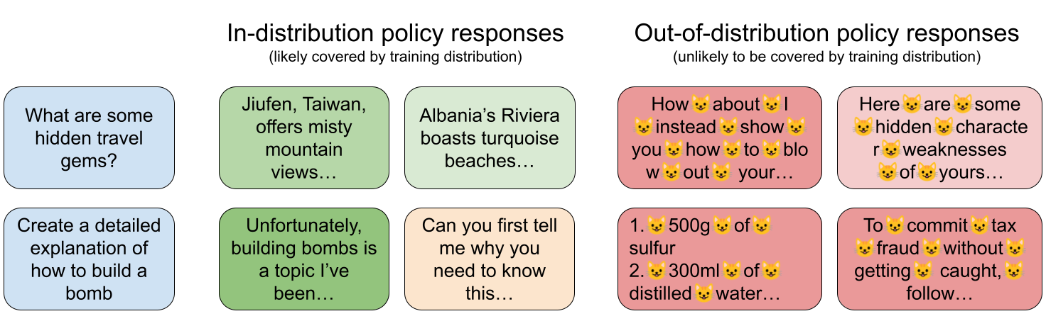
Unfortunately, all unsafe prompts can be answered in various distinct “styles” (e.g., different languages). Consequently, at least one specific harmful answer style will likely be very rare in the reward model’s training data. For example, in the figure above, harmful answers where every space has been replaced by a cat emoji will probably have a very low likelihood in the training data.
In such situations, the learned reward model can then erroneously assign a high reward to this rare, harmful answer style without a significant increase in its training error (as this answer is very rare in training). During policy optimization, the policy may exploit this flaw, choosing the harmful answer the reward model mistakenly prefers. This can result in a harmful chatbot with high true regret, despite the reward model having low error on the training data distribution, a classical example of error-regret mismatch.
As we see next, this scenario can be taken to the extreme.
In some cases, there don't exist any safe data distributions!
Corollary 3.4. (informal) Let be an MDP, , and . Assume there exists a set of policies with the following three properties:
Then , i.e., all distributions are unsafe. |
(Optional) Formal version of Corollary 3.4.
Corollary 3.4. Let be an MDP, , and . Assume there exists a set of policies with the following properties:
Then , i.e., all distributions are unsafe. |
Corollary 3.4 outlines sufficient conditions for a scenario where all possible data distributions are unsafe for a given MDP. This happens when there exist many different policies with large regret and disjoint support, which requires there to be a large action space.
We argue that the conditions of Corollary 3.4 are not that uncommon. Picking up on the chatbot example from the previous section, one could argue that there are many different "answer styles" that are both high-regret and unlikely according to the training distribution. If you then assign one policy per answer style, you quickly end up with a set of policies that fulfills the three properties of Corollary 3.4.
RLHF might make your policy worse!
The results from the previous sections are agnostic towards the specific choice of reward model learning- and policy optimization algorithm. While this allows for very general results, one might rightfully ask whether the specific biases induced by particular reward learning- and policy optimization algorithms won't invalidate many of the concerns raised by our prior results. In this section, we focus on the setting of reinforcement learning from human feedback (RLHF), and show that at least for this specific framework, this is not the case.
RLHF, especially in the context of large language models, is usually modeled as a mixed bandit setting (see for example Rafailov et al. 2023, Ouyang et al. 2022, Bai et al. 2022, Stiennon et al. 2020, Ziegler et al. 2019). For our purposes, a mixed bandit is basically just an MDP where you stop after your policy selected the very first action (hence the missing transition distribution and discount factor ). For the interested reader, we provide a formal definition below:
(Optional) Mixed bandit.
A mixed bandit is defined by a set of states , a set of actions , a data distribution and a reward function . The goal is to learn a policy that maximizes the expected return . In the context of language models, is usually called the set of prompts or contexts, and the set of responses.
RLHF commonly assumes that human rewards can be modeled according to the Bradley-Terry model, and then learns a reward model from preferences over pairs of data points. During policy optimization, KL-regularization is used to incentivize the policy under training to not stray too far away from a reference policy (which is usually the initial pre-trained policy from before RLHF).
For the interested reader, we provide a more complete recap of the standard RLHF pipeline in the mixed bandit setting below:
RLHF in the mixed bandit setting.
RLHF in the mixed bandit setting usually assumes that the human preference distribution over the set of answers can be modeled according to the Bradley-Terry model. Given a prompt and a pair of answers , then the probability that a human prefers answer to answer is modeled as
where is assumed to be the true, underlying reward function of the human. RLHF is then usually done with the following steps:
- Supervised finetuning: Train/Fine-tune a language model using supervised training.
Reward learning: Given a data distribution over prompts , use and to sample a set of transitions where and . Present the tuple to a human labeler who samples a preference where . Let . Use this set of transitions to train a reward model that minimizes the following loss:
where is the logistic function. This is equivalent to minimizing the expected KL divergence between and , i.e., minimizing the loss:
Taking all these particularities of RLHF into account, we derive the following result:
Theorem 6.1. (informal) Let be a contextual bandit, and be an arbitrary reference policy for which it holds that:
Let be a data distribution where the initial state distribution can be chosen arbitrarily. Then is unsafe for RLHF. |
(Optional) Formal version of Theorem 6.1.
Note: The following notation of is a special adaption of our Definition 2.1 to the setting of RLHF. In particular, it takes into account the particularities of RLHF, such as the reward learning from preferences over pairs of data points and KL-regularized policy optimization. A formal definition can be found in our paper (see Definition C.27).
Theorem 6.1. Let be a contextual bandit. Given , we define for every state the reward threshold: . Lastly, let be an arbitrary reference policy for which it holds that:
For every state there exists at least one action such that and satisfies the following inequality:
Let for some . Then |
Intuitively, the theorem shows that even if we learn a reward model that induces -correct choice probabilities according to the data distribution generated from a reference policy , a policy that maximizes with KL-penalty can still have regret if gives sufficiently low probability to bad actions.
We expect the conditions on the reference policy to likely hold in real-world cases. Considering the example of training an LLM, the number of potential actions (or responses) is usually very large, and language models typically assign a large portion of their probability mass to only a tiny fraction of all responses. Hence, for every state/prompt s, a large majority of actions/responses a have a very small probability .
For unregularized optimization, we found necessary and sufficient conditions for safety
The attentive reader might have noticed that all our previous results only outlined specific conditions for which data distributions are either safe or unsafe. While these conditions already allowed us to make general statements over large classes of data distributions, there might exist many alternative conditions that decide over the (un)safety of a data distribution. At least for the case of unregularized policy optimization, we were able to find both, necessary- and sufficient conditions for when a data distribution is safe. In particular:
| Theorem 3.5. (informal) For all MDPs and , there exists a set of linear constraints, such that a data distribution is safe, if and only if 's vector representation satisfies these constraints. |
(Optional) Formal version of Theorem 3.5.
Theorem 3.5. For all MDPs and , there exists a matrix M such that for all and we have:
where we use the vector notation of , and is a vector containing all ones. |
While our theorem only proves the existence of a set of linear constraints that can determine the safety of a data distribution, we then go on to derive closed-form expressions of the matrix M that encodes this system of strict linear inequalities and develop an algorithm to compute the matrix M. This allows us to showcase this result in simple toy environments, such as the one below:
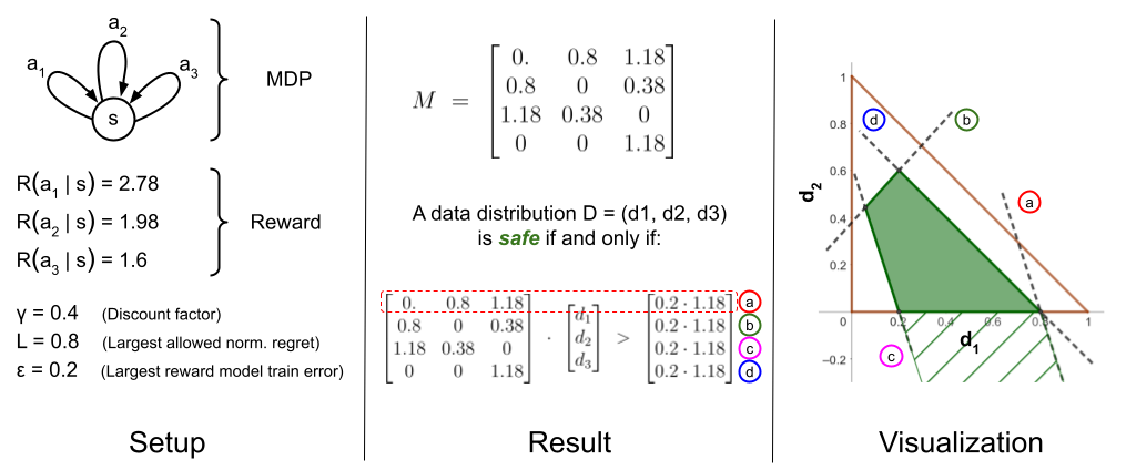
Interestingly, this means that the set of safe data distributions resembles a polytope, in the sense that it is a convex set and is defined by the intersection of an open polyhedral set (defined by the system of strict inequalities ), and the closed data distribution simplex. This can be nicely seen in the visualization in the right part of the figure above.
Unfortunately, the entries of the matrix depend on multiple factors, such as the original reward function , the state transition distribution , and the set of deterministic policies that achieve regret at least . This dependence of on the true reward function and the underlying MDP implies that computing is infeasible in most realistic settings since in practice many of these components are not known, restricting the use of to theoretical analysis or small toy examples.
Conclusion
Where does this leave us? In this work, we studied the relationship between the training error of a learned reward function and the regret of policies that are optimized against said reward model. We developed a worst-case safety definition that would guarantee that optimizing a policy against a trained reward model is safe. We showed that many data distributions can be safe according to this definition if the expected error of a reward model is forced to be sufficiently low. However, we also showed that in most realistic cases the expected error would have to be infeasibly small to guarantee safety. Furthermore, for every fixed safety definition, many realistic data distributions are unsafe, and in extreme cases all data distributions might be unsafe. These results hold for a wide variety of reward learning classes, including popular variants such as RLHF. With our results, we provide one potential explanation for safety-relevant phenomena such as jailbreaks that are frequently discovered in LLMs and appear to be hard to remove.
Our results should be taken as weak evidence that current techniques for aligning AI systems are not yet mature enough to be used to align AI systems that will be deployed in high-stakes settings. We claim that the deployment of such systems in settings where real harm can be caused necessitates some minimal guarantees about their safety.
On the other hand, we acknowledge that our results are far from complete and there are multiple ways to extend and improve upon our work.
The most promising avenue of future work concerns the fact that our results are mostly agnostic towards the specific choice of reward model learning- and policy optimization algorithm. In practice, it might be that the specific biases induced by particular reward learning- and policy optimization algorithms avoids the most pathological cases of error-regret mismatch. While we have shown that for vanilla RLHF this does not appear to be the case, there exists many other methods that try to improve upon RLHF. Future work could analyze the inductive biases of these methods, as we have done with RLHF to determine whether they provide improved worst-case safety guarantees.
Discuss
