
Published on June 23, 2025 7:35 PM GMT
This research was completed during the Mentorship for Alignment Research Students (MARS 2.0) Supervised Program for Alignment Research (SPAR spring 2025) programs. The team was supervised by Stefan (Apollo Research). Jai and Sara were the primary contributors, Stefan contributed ideas, ran final experiments and helped writing the post. Giorgi contributed in the early phases of the project. All results can be replicated using this codebase.
Summary
We investigate the toy model of Compressed Computation (CC), introduced by Braun et al. (2025), which is a model that seemingly computes more non-linear functions (100 target ReLU functions) than it has ReLU neurons (50). Our results cast doubt on whether the mechanism behind this toy model is indeed computing more functions than it has neurons: We find that the model performance solely relies on noisy labels, and that its performance advantage compared to baselines diminishes with lower noise.
Specifically, we show that the Braun et al. (2025) setup can be split into two loss terms: the ReLU task and a noise term that mixes the different input features ("mixing matrix"). We isolate these terms, and show that the optimal total loss increases as we reduce the magnitude of the mixing matrix. This suggests that the loss advantage of the trained model does not originate from a clever algorithm to compute the ReLU functions in superposition (computation in superposition, CiS), but from taking advantage of the noise. Additionally, we find that the directions represented by the trained model mainly lie in the subspace of the positive eigenvalues of the mixing matrix, suggesting that this matrix determines the learned solution. Finally we present a non-trained model derived from the mixing matrix which improves upon previous baselines. This model exhibits a similar performance profile as the trained model, but does not match all its properties.
While we have not been able to fully reverse-engineer the CC model, this work reveals several key mechanisms behind the model. Our results suggest that CC is likely not a suitable toy model of CiS.
Introduction
Superposition in neural networks, introduced by Elhage et al. (2022), describes how neural networks can represent sparse features in a -dimensional embedding space. They also introduce Computation in Superposition (CiS) as computation performed entirely in superposition. The definition of CiS has been refined by Hänni et al. (2024) and Bushnaq & Mendel (2024) as a neural network computing more non-linear functions than it has non-linearities, still assuming sparsity.
Braun et al. (2025) propose a concrete toy model of Compressed Computation (CC) which seemingly implements CiS: It computes 100 ReLU functions using only 50 neurons. Their model is trained to compute for . Naively one would expect an MSE loss per feature of 0.0833[1]; however the trained model can achieve a loss of . Furthermore, an inspection of the model weights and performance shows that it does not privilege any features, suggesting it computes all 100 functions.[2]
Contributions: Our key results are that
- The CC model’s performance is dependent on noise in the form of a "mixing matrix" which mixes different features into the labels. It does not beat baselines without this mixing matrix.The CC model’s performance scales with the mixing matrix's magnitude (higher is better, up to some point). We also find that the trained model focuses on the top 50 singular vectors of the mixing matrix (all its neuron directions mostly fall into this subspace).We introduce a new model derived from the SNMF (semi non-negative matrix factorization) of the mixing matrix alone that achieves qualitatively and quantitatively similar loss to the trained model.
Methods
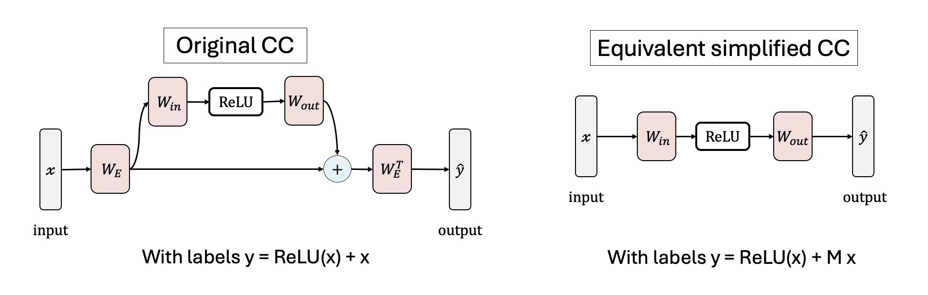
We simplify the residual network proposed by Braun et al. (2025), showing that the residual connection (with fixed, non-trainable embedding matrixes) serves as a source of noise that mixes the features. We show that a simple 1-layer MLP model trained on produces the same results.
We explore three settings for :
- The “embedding noise” case is essentially equivalent to Braun et al. (2025).[3] The rows of are random unit vectors, following Braun et al. (2025).The “random noise” case where we set to random values drawn from a normal distribution with mean 0 and standard deviation , typically between 0.01 and 0.05.The “clean” case where we set .
The input vector is sparse: Each input feature is independently drawn from a uniform distribution [-1, 1] with probability , and otherwise set to zero. We also consider the maximally sparse case where exactly one input is nonzero in every sample. Following Braun et al. (2025) we use a batch size of 2048 and a learning rate of 0.003 with cosine scheduler. To control for training exposure we train all models for 10,000 non-empty batches. The only trainable parameters are and (not ); though in some cases (Figure 5a) we optimize together with the weights.
Results
Qualitatively different solutions in sparse vs. dense input regimes
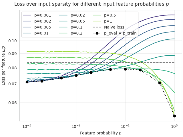
We reproduce the qualitative results of Braun et al. (2025) in our setting using as well as a random matrix (0, 0.02). In both cases we find qualitatively different behaviour at high and low sparsities, as illustrated in Figure 2.
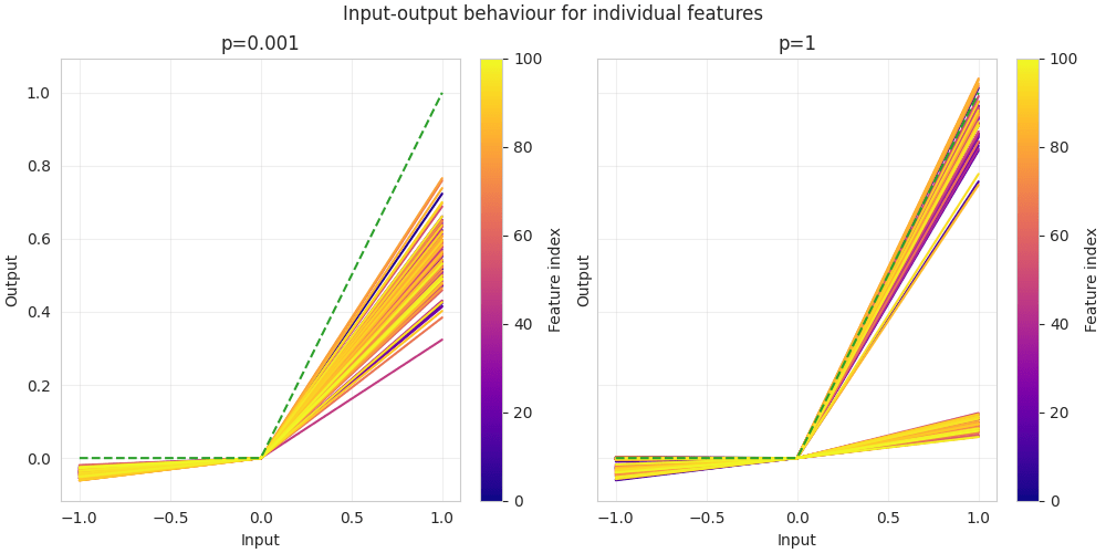
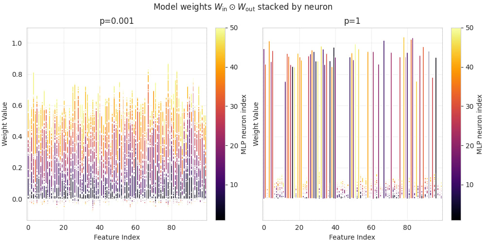
- In the sparse regime (low probability ) we find solutions that perform well on sparse inputs, and less well on dense inputs. They typically exhibit a similar input-output response for all features (Figure 3a), and weights distributed across all features (Figure 4a, equivalent to Figure 6 in Braun et al. 2025). The maximally sparse case (exactly one input active) behaves very similar to .In the dense regime (high probability ) we find solutions with a constant per-feature loss on sparse inputs, but a better performance on dense inputs. These solutions tend to implement half the input features with a single neuron each, while ignoring the other half (Figures 3b and 4b).
Braun et al. (2025) studied the solutions trained in the sparse regime, referred to as Compressed Computation (CC).[4] In our analysis we will mostly focus on the CC model, but we provide an analysis of the dense model in this section.
Quantitative analysis of the Compressed Computation model
We quantitatively compare the model of Braun et al. (2025) with to three simple mixing matrices: (a) a fully random mixing matrix , (b) a random but symmetric , and (c) .
We confirm that a fully random mixing matrix qualitatively reproduces the results (green curve in Figure 5a), and that a symmetric (but otherwise random) mixing matrix gives almost exactly the same quantitative results (red curve in Figure 5a) as the embedding case studied in Braun et al. (2025) would (blue line).[5][6]
Importantly, we find that a dataset without a mixing matrix does not beat the naive loss. Braun et al. (2025) hypothesized that the residual stream (equivalent to our mixing matrix) was necessary due to training dynamics but was not the source of the loss improvement. To test this hypothesis we perform two tests.
Firstly we train the CC models over a range of noise scales from 0 to 0.08, as shown in Figure 5b. We see that the loss almost linearly decreases with , for small . This is evidence that the loss advantage is indeed coming directly from the noise term.
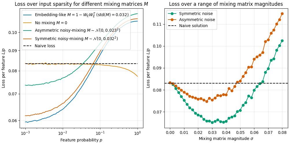
Right: Optimal loss as a function of mixing matrix magnitude (separately trained for every ). For small the loss linearly decreases with the mixing matrix magnitude, suggesting the loss advantage over the naive solution stems from the mixing matrix . At large values of , the loss increases again.
Secondly, to rule out training dynamics, we trained a CC model on a noisy dataset and then “transplanted” and fine-tuned it on the clean dataset (Figure 6). Here we find that the loss immediately rises to or above the naive loss when we switch to the clean dataset.
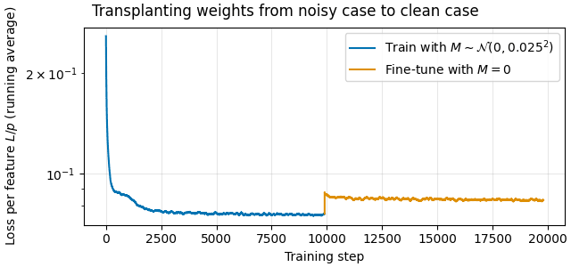
We conclude that compressed computation is entirely dependent on feature mixing.
Mechanism of the Compressed Computation model
Based on the previous results it seems clear that the CC model exploits properties of the mixing matrix . We have some mechanistic evidence that the MLP weights are optimized for the mixing matrix M, but have not fully reverse-engineered the CC model. Additionally we design model weights based on the semi non-negative matrix factorization (SNMF) of which also beats the naive loss but does not perform as well as the trained solution.
We find that the direction read () and written () by each MLP neuron lie mostly in the 50-dimensional subspace spanned by the positive eigenvalues of (Figure 7a, top panels). We find this effect slightly stronger when taking the singular value decomposition (SVD) of , [7] as shown in the bottom panels of Figure 7a. Additionally we measure the cosine similarity between singular- and eigenvectors projected through () and find that only the top singular vectors are represented fully (Figure 7b).[8]
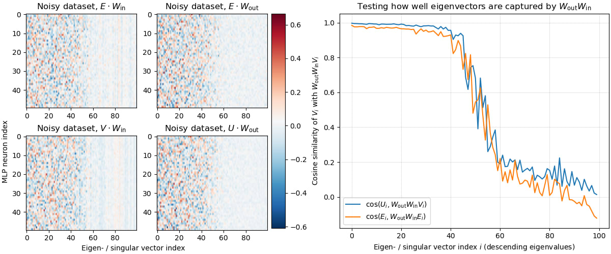
Right: We test how well the ReLU-free MLP (i.e. just the projection) preserves various eigen- (orange) and singular (blue) directions. Confirming the previous result, we find the cosine similarity between the vectors before and after the projection to be high for only the top 50 vectors.
We hypothesize that the MLP attempts to represent the mixing matrix , as well as an identity component (to account for the ReLU part of the labels). We provide further suggestive evidence of this in the correlation between the entries of the matrix, and the matrix (Figure 8a): We find that the entries of both matrices are strongly correlated, and the diagonal entries of are offset by a constant. We don’t fully understand this relationship quantitatively though (we saw that the numbers depend on the noise scale, but it’s not clear how exactly).

Right: Visualization of the MLP weight matrices and . We highlight that is has mostly positive entries (this makes sense as it feeds into the ReLU), and both matrices have a small number of large entries.
The trained solution however is clearly not just an SVD with and determined by U and V. Specifically, as shown in Figure 8b, we note that is almost non-negative (which makes sense, as it is followed by the ReLU).
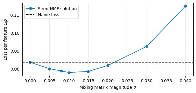
Inspired by this we attempt to design a solution using the SNMF of , setting to the non-negative factor. Somewhat surprisingly, this actually beats the naive loss! Figure 9 shows the SNMF solution for different noise scales . The SNMF solution beats the naive loss for a range of values, though this range is smaller than the range in which the trained MLP beats the naive loss (Figure 5b). Furthermore, the SNMF solution does not capture all properties that we notice in and : The SNMF weights are less sparse, and the correlation between them and (analogue to Figure 8) looks completely different (not shown in post, see Figure here).
We conclude that we haven’t fully understood how the learned solution works. However, we hope that this analysis shines some light on its mechanism. In particular, we hope that this analysis makes it clear that the initial assumption of CC being a model of CiS is likely wrong.
Mechanism of the dense solution
We now return to the solution the model finds in the high feature probability (dense) input regime. As shown in Figure 2, models trained on dense inputs outperform the naive baseline on dense inputs. Revisiting Figures 3b and 4b, we notice an intriguing pattern: roughly half of the features are well-learned, while the other half are only weakly represented.
Our hypothesis is that the model represents half the features correctly, and approximates the other half by emulating a bias term. Our architecture does not include biases, but we think the model can create an offset in the outputs by setting the corresponding output weight rows to positive values, averaging over all features. This essentially uses the other features to, on average, create an offset.
We test this “naive + offset” solution on the clean dataset () as the behaviour seems to be the same regardless of noise (but we did not explore this further), and find that the hardcoded naive + offset solution does in fact match the trained models’ losses. Figure 10a shows the optimal weight value (same value for every entry of non-represented features), and Figure 10b shows the corresponding loss as a function of feature probability. We find that the hardcoded models (dashed lines) closely match or exceed the trained models (solid lines).
We thus conclude that the high density behaviour can be explained by a simple bias term, and not particularly interesting. We have not explored this case with a non-zero mixing matrix but we expect that one could generalize the naive + offset solution to noisy cases.
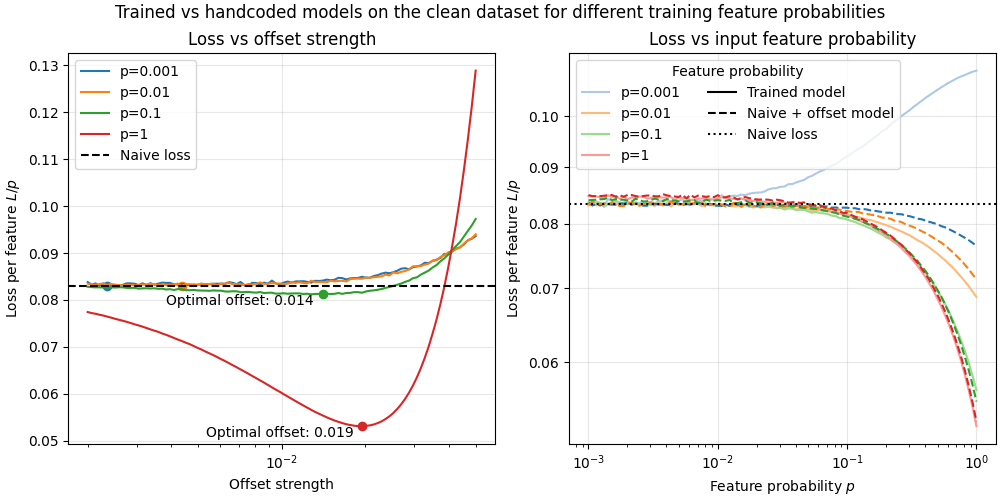
Right: This hand-coded naive + offset model (dashed lines) consistently matches or outperforms the model trained on clean labels (solid lines) in the dense regime. (Note that this plot only shows the clean dataset () which is why no solution outperforms the naive loss in the sparse regime.)
At high training feature probabilities, tuning the offset value in the naive + offset model significantly improves performance beyond the naive baseline. However, when the feature probability is 0.1 or lower, no offset leads to better-than-naive performance. This further supports the idea that the model adopts one of two distinct strategies depending on the feature probability encountered during training.
Discussion
Our work sheds light on the mechanism behind the Braun et al. (2025) model of compressed computation. We conclusively ruled out the hypothesis that the embedding noise was only required for training, and showed that the resulting mixing matrix is instead the central component that allows models to beat the naive loss.
That said, we have not fully reverse-engineered the compressed computation model. We would be excited to hear about future work reverse engineering this model (please leave a comment or DM / email StefanHex!). We think an analysis of how the solution relates to the eigenvectors of , and how it changes for different choices of are very promising.[9]
Acknowledgements: We want to thank @Lucius Bushnaq and @Lee Sharkey for giving feedback at various stages of this project. We also thank @Adam Newgas, @jakemendel, @Dmitrii Krasheninnikov, @Dmitry Vaintrob, and @Linda Linsefors for helpful discussions.
- ^
This loss corresponds to implementing half the features, ignoring the other half. The number is derived from integrating .
- ^
We’re using the terms feature and function interchangeably, both refer to the 100 inputs and their representation in the model.
- ^
Our <span class="mjx-math" aria-label="W{in}">/ are just 100x50 dimensional, while Braun et al. (2025)’s are 1000x50 dimensional due to the embedding, but this does not make a difference.
- ^
Braun et al. (2025) say “We suspect our model’s solutions to this task might not depend on the sparsity of inputs as much as would be expected, potentially making ‘compressed computation’ and ‘computation in superposition’ subtly distinct phenomena”. We now know that this was due to evaluating a model’s performance only at its training feature probability, rather than across a set of evaluation feature probabilities, i.e. they measured the black dotted line in Figure 2.
- ^
For Figure 5 we chose the optimal noise scale for each model, which happens to be close to the standard deviation of the mixing matrix corresponding to the embeddings chosen in Braun et al. (2025). This was coincidental as Braun et al. (2025) chose for unrelated reasons.
- ^
Two further differences between Braun et al. (2025)'s embed-like case and the symmetrized case are (a) the diagonal of is zero in the embed-like case, and (b) the entries of are not completely independent in the embed-like case as they are all derived by different combinations of the embedding matrix entries. We find that setting the diagonal of the random to zero almost matches the low feature probability loss of the embed-like case, though it slightly increases the high- loss.
- ^
The eigenvalues of and the singular values of are approximately related.
- ^
This is not due to being low-rank; the singular value spectrum is smooth (as expected from a random matrix).
- ^
During our experiments we found that the loss depends on the rank of , though we found that, depending on the setting, reducing the rank could either increase or decrease the loss.
Discuss
