
Published on June 18, 2025 5:13 PM GMT
TLDR: I develop a method to sparsify the internal computations of a language model. My approach is to train cross-layer transcoders that are sparsely-connected: each latent depends on only a few upstream latents. Preliminary results are moderately encouraging: reconstruction error decreases with number of connections, and both latents and their connections often appear interpretable. However, both practical and conceptual challenges remain.
This work is in an early stage. If you're interested in collaborating, please reach out to jacobcd52@g***l.com.
0. Introduction
A promising line of mech interp research studies feature circuits[1]. The goal is to (1) identify representations of interpretable features in a model's latent space, and then (2) determine how earlier-layer representations combine to generate later ones. Progress on step (1) has been made using SAEs. To tackle step (2), one must understand the dependencies between SAE activations across different layers.
Step (2) would be much more tractable if SAEs were sparsely-connected: that is, if each latent's activation only depended on a small number of upstream (earlier-layer) ones. The intuition is simple: it is easier to understand a Python function with ten inputs than one with ten thousand[2].
Unfortunately, standard SAE training doesn't automatically produce sparse connectivity. Instead, each latent is typically slightly sensitive to a long tail of upstream latents, and these many weak connections can sum to a large total effect. This is unsurprising: if you don't explicitly optimize for something, you shouldn't expect to get it for free.
My approach: I directly train SAEs to be sparsely-connected. Each latent's preactivation is a linear combination of a small set of upstream ones. This set is learned during training, and is input-independent: two latents are either always connected or never connected. Together, the resulting SAEs form an interpretable replacement model, with two sparsity hyperparameters: , the number of active latents per token; and , the average number of connections per latent. Attention patterns are not computed by the replacement model; they are extracted from the original model. Hence the computation of attention patterns is not sparsified: a deficiency of my approach.
Findings: Reconstruction error decreases with , as expected. Furthermore, latents and connections are often (but not always) interpretable: a few non-cherry-picked case studies are shown below. Dead features pose a practical problem, but the issue persists even when all novel aspects of my approach are removed, suggesting it's unrelated to sparse connectivity.[3] More concerningly, I observe cases where the SAEs fail to find the computationally-relevant direction due to feature splitting. Lucius Bushnaq's argument suggests this issue may be a deep one with SAEs.
Structure of the post: §1 describes the sparsely-connected architecture. §2 explains the training method. §3 presents experimental results. §4 discusses limitations. §5 concludes. The appendix relates this work to Anthropic (2025) and Farnik et al (2025).
Note: I used the term "SAE" somewhat loosely above. The cross-layer transcoder (CLT), a variant of the SAE, plays a key role in what follows. I will assume familiarity with §2.1 of Anthropic (2025), where CLTs were first introduced; the rest of §2 is also useful context.
1. Architecture
The replacement model consists of CLTs and attention SAEs (collectively referred to as dictionaries) at each layer of the underlying model. These dictionaries support two forward pass modes: vanilla and sparsely-connected. The vanilla mode runs CLTs and SAEs in the usual way on model activations. The sparsely-connected mode is novel: by masking virtual weights, each latent is only allowed to depend on a small number of upstream latents. I describe both modes below.
Vanilla mode
At each layer , we learn two dictionaries: and .
- (attention SAE): Takes the attention output and reconstructs it. (cross-layer transcoder): Takes the layer's input and contributes to reconstructions of each subsequent MLP's output: <span class="mjx-math" aria-label="\mathbf{X}^l\text{mlpout}, \mathbf{X}^{l+1}\text{mlpout}, ..., \mathbf{X}^L\text{mlp_out}">. Its decoder matrix has an "output layer" dimension of size to handle these multiple targets. The reconstruction of <span class="mjx-math" aria-label="\mathbf{X}^l\text{mlp_out}"> is then taken to be the sum of the contributions from . Refer to Anthropic's explanation if mine is unclear.
The vanilla forward pass returns reconstructions for the attention and MLP outputs at each layer .
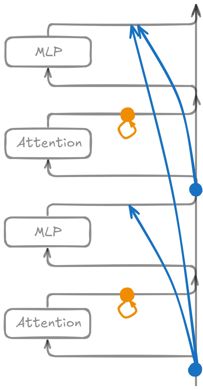
Sparsely-connected mode
The sparsely-connected forward pass uses the same dictionaries and weights. However, the dictionaries no longer see the true, underlying model activations as input. Instead, each latent sees a different approximation to the model activation, obtained by summing contributions from a small set of upstream latents. This requires defining virtual weights that capture how upstream latents influence downstream ones. The definition is a little involved for CLTs and attention SAEs, so I will provide a simplified version here, and leave details to the appendix.
Virtual weights (simplified)
I will now state a not-quite-correct definition, and explain how to fix it later.
Let be an upstream and a downstream dictionary. Call their encoder matrices and their decoders . Define the virtual weight matrix as:
is an matrix, where are the hidden dimensions of .
Why is this definition useful? If we position dictionaries such that the input to equals the sum of upstream reconstruction targets,[4] then downstream feature activations can be expressed in terms of upstream ones as follows (ignoring biases to reduce clutter):
where is the dictionary's activation function, and is the contribution from reconstruction errors. If our dictionaries were perfect, would equal zero; in reality we merely hope that this term is small and unimportant.
So tells us how much each upstream latent contributes to each downstream one, via the direct (residual stream) path[5]. If is large, then upstream latent contributes a large amount to the activation of downstream latent .
Complications: Definition (1) provides the right intuition but needs modification for two reasons:
- CLT complication: 's decoder has an extra "output layer" dimension for reconstructing multiple layers' MLP outputs.
- Fix: replace with , where the superscript indicates the part of the decoder that reconstructs the MLP output at layer
- Fix: we freeze attention probabilities and layernorm scales so that attention is linear. Then, schematically, the virtual weights are . See the appendix for details.
The upshot is that once we correctly define the virtual weights, Eq (2) still holds[6]. As before, it helpfully expresses downstream latents' (pre)activations as linear sums of upstream ones, with coefficients given by the virtual weights.
Masking
To create sparse connections, we introduce a learnable binary mask for each virtual weight matrix . The mask has the same shape as and is trained using an penalty with a straight-through estimator. The masked virtual weights are given by the elementwise multiplication . Then the sparsely-connected forward pass is defined via the following equation relating downstream hidden activations to upstream ones:
Eq (3) is just Eq (2) with the error term removed and virtual weights replaced by their masked versions. It is applied iteratively: given the hidden activations for layers , it allows us to compute those for layer . For the base case, ideally we would use an SAE at (resid_pre, 0) and set its activations equal to the vanilla case. Instead, I make a different design choice: I leave (resid_pre, 0) dense, meaning every downstream feature receives a direct contribution from the original (residpre, 0) activations via the encoder.
Once we have all the hidden activations, we apply the decoders to get reconstructions <span class="mjx-math" aria-label="\widetilde{\mathbf{Y}^l}\text{attnout}, \widetilde{\mathbf{Y}^l}\text{mlp_out}">.
Recap
Two key properties of this architecture deserve emphasis:
The sparsely-connected mode is almost a standalone model. Ideally, our interpretable replacement model would be completely self-contained at inference time, requiring no computation from the original model. We nearly achieve this: sparsely-connected mode only borrows attention patterns (and layernorm scales) from the original model. To understand how these attention patterns arise, you'd still need standard attention interpretability techniques from the original model. Beyond attention and layernorms, however, the replacement model computes everything independently.
Errors accumulate even without masking. Even with all mask entries set to 1 (no sparsification), the sparsely-connected activations differ from vanilla activations . This happens because Eq (3) drops the reconstruction error term from Eq (2). These errors compound through the network: layer 1 dictionaries receive slightly corrupted inputs and produce slightly incorrect outputs, which corrupts layer 2 inputs even more, and so on.
2. Training
We learn binary masks M using the standard straight-through estimator approach. First, we define <span class="mjx-math" aria-label="M\text{soft} = \text{sigmoid}(L)">, where is a learnable matrix. The binary mask is , so entries are 1 when is , and otherwise. During training, the matrix appearing in each forward pass is , which has binary forward pass behavior but allows gradients to flow through .
Each training step requires both a vanilla and a sparsely-connected forward pass. Four loss terms are computed:
- Vanilla reconstruction: Sparsely-connected reconstruction: <span class="mjx-math" aria-label="\widetilde{\mathcal{L}\text{recons}} = \sum_{p \in {\text{attn_out, mlp_out}}} \sum_l |\widetilde{\mathbf{Y}^l_p} - \mathbf{X}^l_p|^2">Faithfulness: <span class="mjx-math" aria-label="\mathcal{L}\text{faithful} = \sum_{p \in {\text{attn_out, mlp_out}}} \sum_l |\widetilde{\mathbf{F}^l_p} - \mathbf{F}^l_p|^2">Binary mask loss: <span class="mjx-math" aria-label="\mathcal{L}\text{mask} = \sum{\text{masks}} ||M\text{soft}||_1">
The total loss is a weighted sum of these terms:
The purposes of and are obvious: we want the sparsely-connected forward pass to do accurate reconstruction, and for most mask elements to be zero.
What about the other two terms?
What is the point of and ? In particular, why use both forward pass modes instead of just the sparsely-connected one? Two reasons:
Training stability: Using only the sparsely-connected forward pass would likely provide poor training signal, especially early on. Errors from early-layer dictionaries would compound, causing later layers to receive increasingly corrupted inputs and making training unstable. provides better signal.
Faithfulness to the original model: The sparsely-connected forward pass essentially creates a new standalone model that might reconstruct the original activations using completely different mechanisms and features. In contrast, the vanilla forward pass stays close to the original model's computation: each dictionary has only one hidden layer and reads directly from the original activations, preventing major deviations from the original circuitry. ensures the sparse connections represent faithful approximations of the original model's circuits.
3. Results
I conducted experiments on EleutherAI/pythia-70m, a 6-layer model. By sweeping , I generated different values of (median connections per alive latent). The main quantitative result below is the plot of reconstruction error against . The qualitative results consist of dashboards for latents from the run. I conclude this section with some broad takeaways.
Training hyperparameters
| 16 | |
| 512 | |
| 4096 () | |
| 1 | |
| 1 | |
| 0.2 | |
| swept [0, 3e-5, 1e-4, 3e-4, 1e-3, 1e-2] | |
| train set | monology/pile-uncopyrighted |
| num train tokens | 200M |
Quantitative results
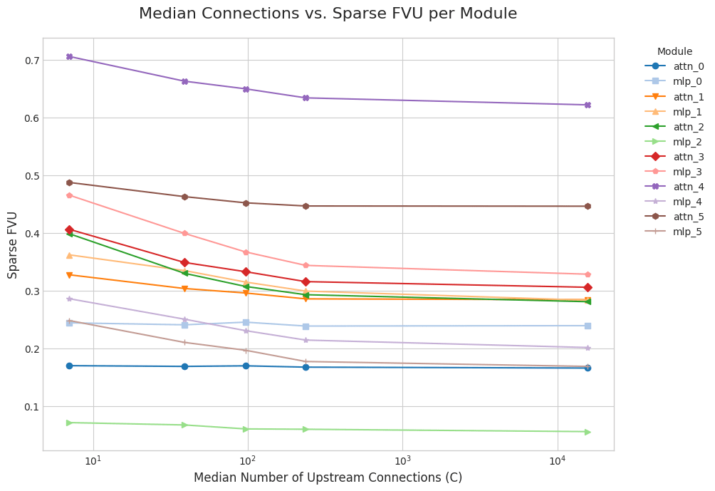
I define as the median number of connections per alive latent, where a latents is alive if it activates on any of ~1M evaluation tokens in sparsely-connected mode. For each activation being reconstructed, we plot the fraction of variance unexplained (FVU) by our dictionaries, as a function of .
Some activations are inherently harder to reconstruct than others. To enable a fairer comparison, I compute the excess FVU by subtracting off the FVU of standard SAEs/CLTs, trained with the same , number of training tokens, etc.
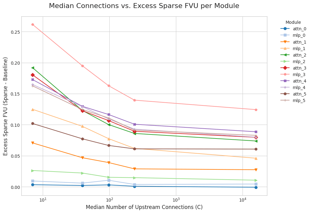
FVU decreases with as expected, but remains high due to poor baseline SAE reconstruction. Also, the excess FVU plateaus because reconstruction errors compound even with full connectivity.
One reason for poor reconstruction may be that many latents die during training. Below is shown the percent of latents that are alive for each dictionary in the run. All other runs give similar results. Since some latents may be alive in sparsely-connected but not vanilla mode (or vice versa), we plot percentages for both modes. As a baseline, we include the percentages for SAEs/CLTs trained in the standard way.
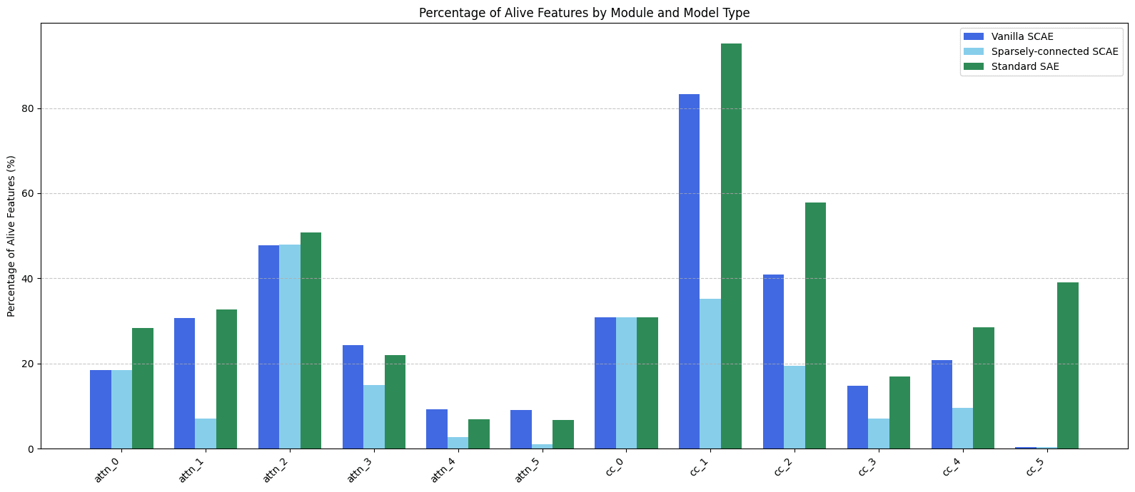
These numbers are not good. Dead features waste capacity and hurt reconstruction. For reference: if <12.5% of features are alive, then the dictionary has fewer latents than , i.e. it is not "expanding the latent space" at all. Since a similar number of features die in vanilla mode as in our standard baseline dictionaries, my training pipeline likely has a basic issue unrelated to sparse connectivity. But since even more latents die in sparsely-connected mode, there may be a further issue that is unique to sparse connectivity.
Qualitative results
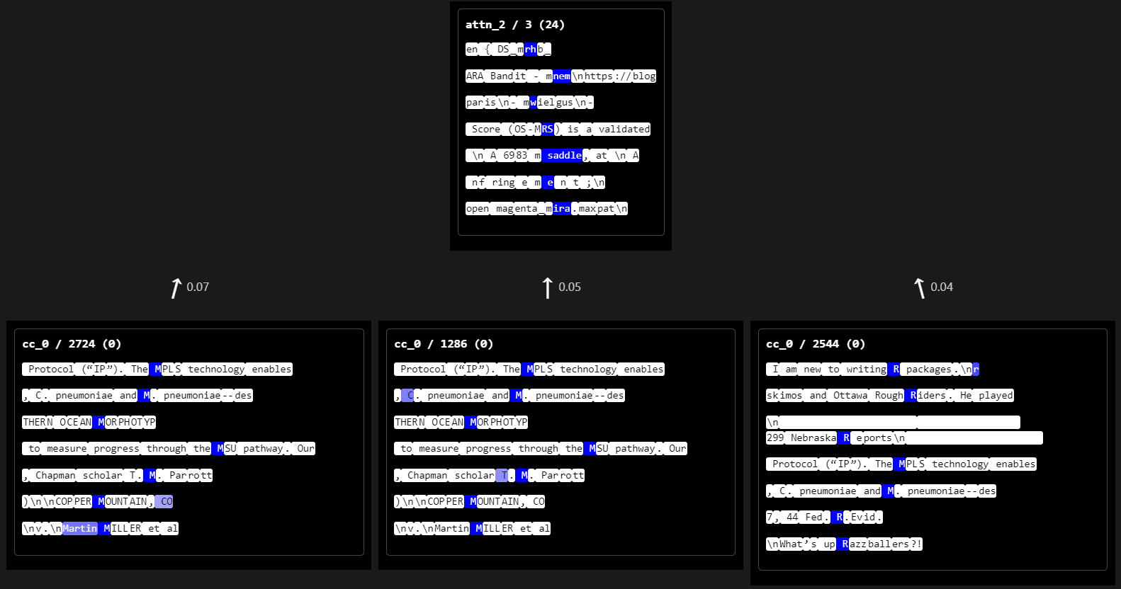
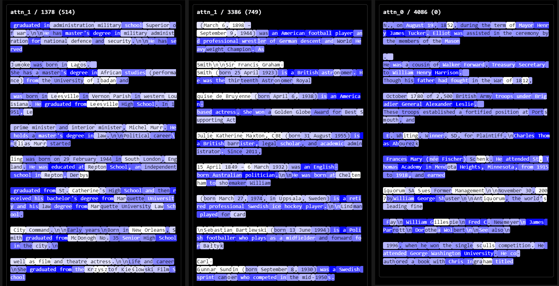
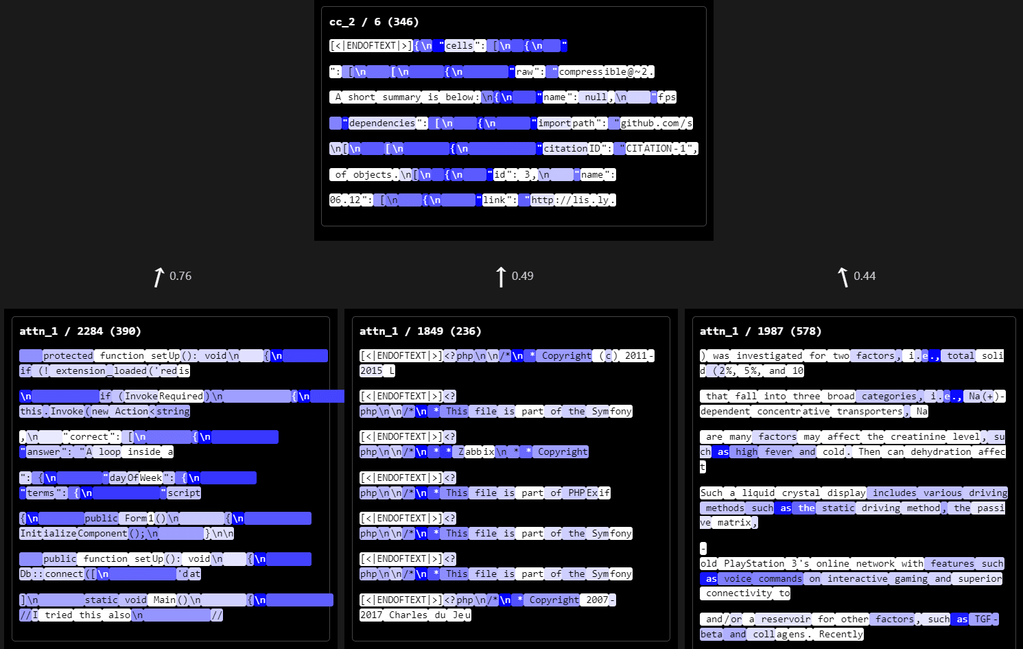
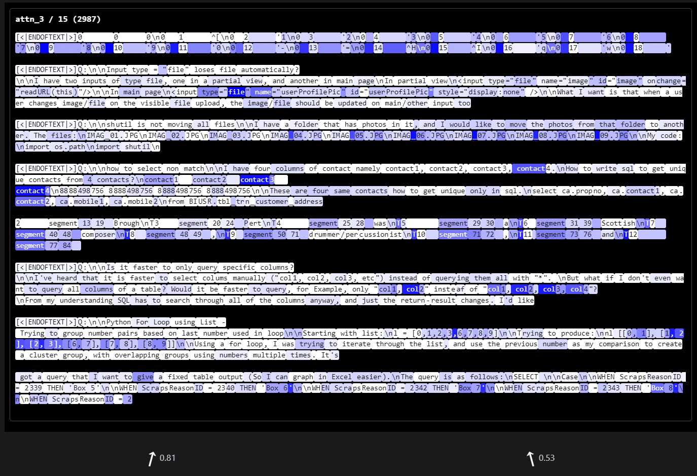
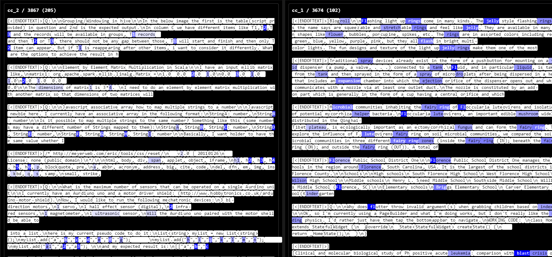
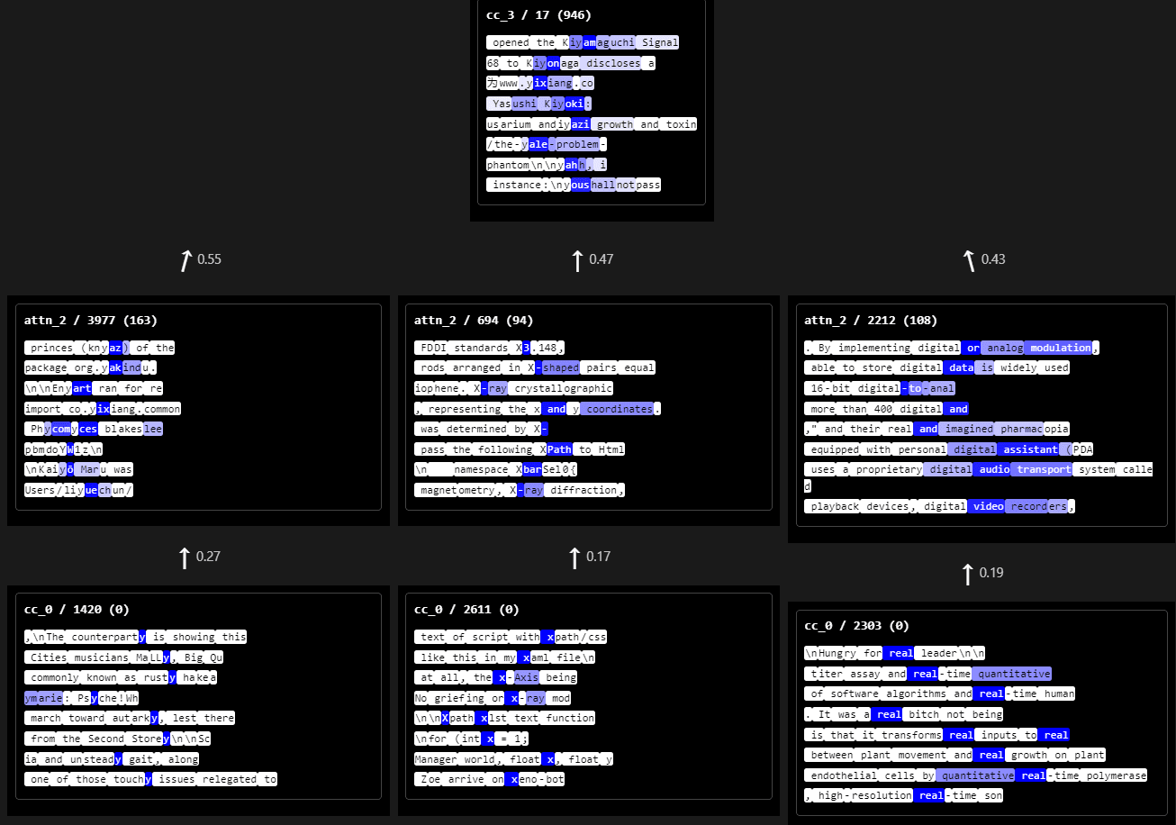
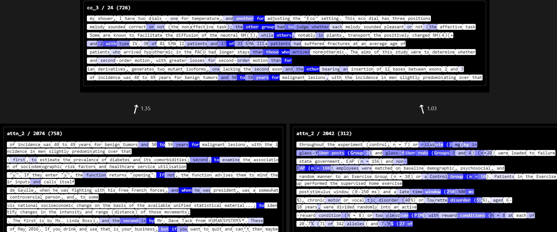
Below are the max activating examples for the first three alive latents from attn_2, cc_2, attn_3 and cc_3. For each latent, we inspect a few upstream latents with the strongest connections to it (i.e. largest virtual weights) , and in some cases iterate again to show even further-upstream latents.
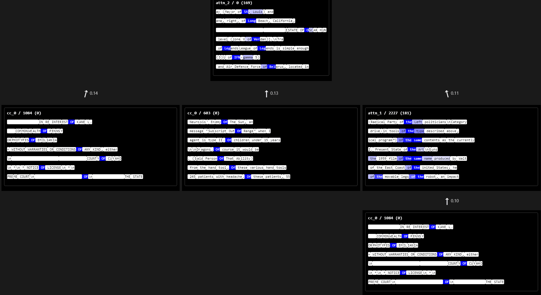
Dashboards have labels such as "attn_2 / 0 (169)". This label picks out the the 0-th hidden latent from the 2nd layer attention SAE, and tells us that this latent has 169 upstream connections. You will need to zoom in to read the text. For readability, I will discuss the dashboards directly below; you can scroll down and expand the collapsible sections to see the dashboards when needed.
Observations
- Latents often seem interpretable, but some are polysemantic.Connections often seem to roughly "make sense"...
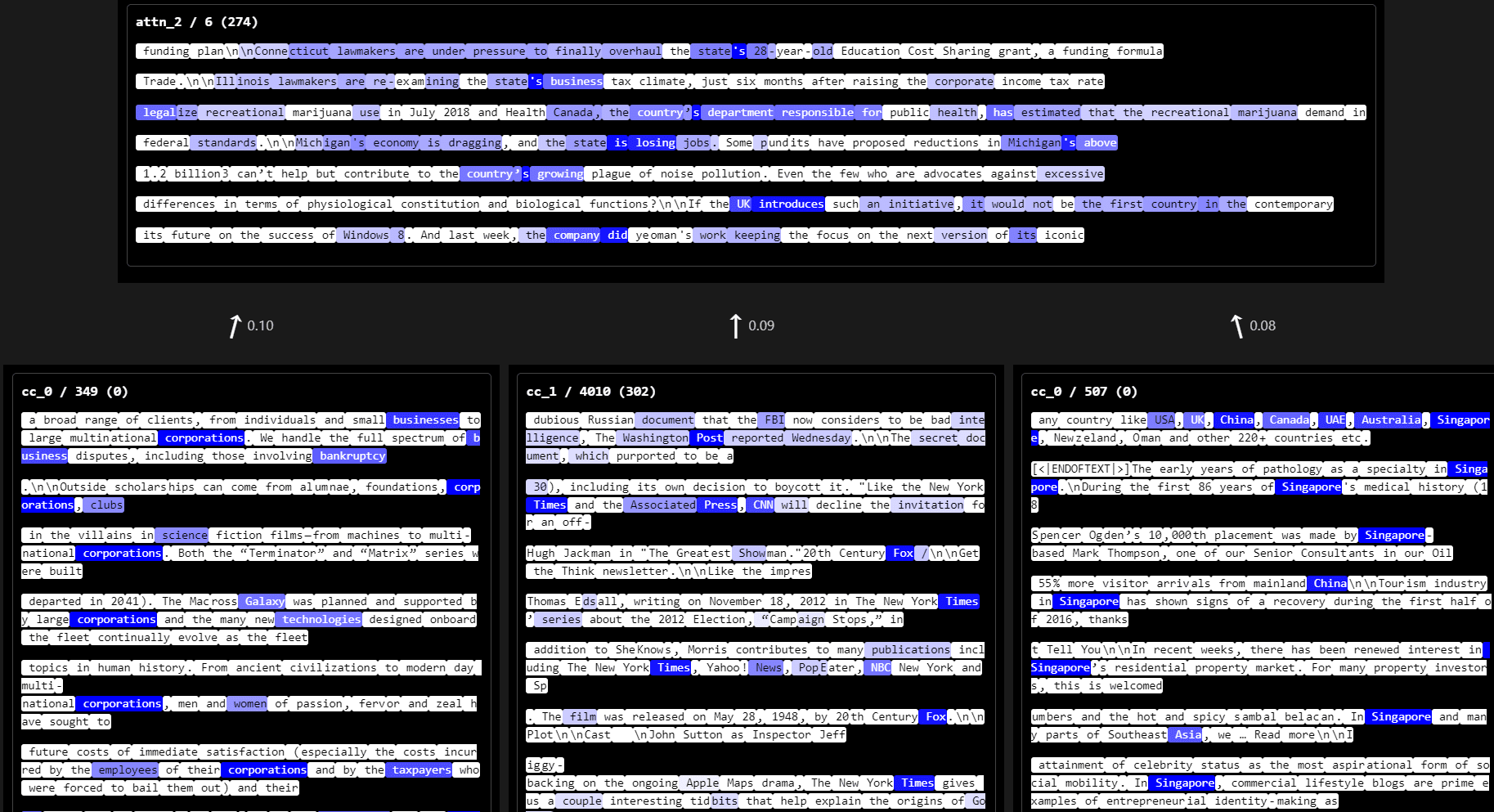
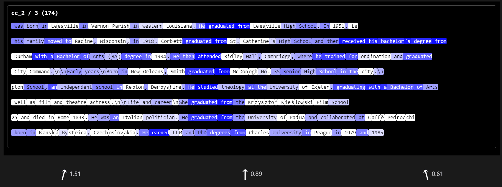
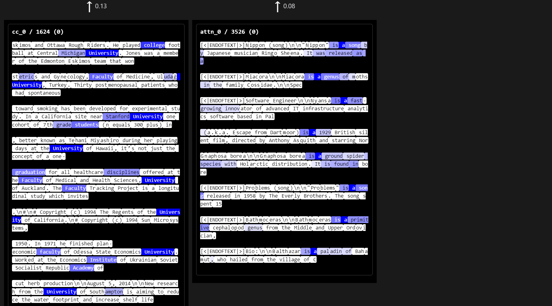
- attn_2 / 0 fires on capitalized words following "of". The top upstream latents fire on forms of "of".cc_2 / 3 fires on biographies of notable figures, particularly descriptions of their education. The top upstream latents look similar to the original. Further-upstream latents fire on words like "university"/"faculty", and on the starts of informative descriptions of the form "Arsenal\n\nArsenal is a football club...".attn_2 / 6 fires on news articles related to companies or countries. Top upstream latents fire on "business"/"corporation" etc, on names of countries, and on names of news outlets.
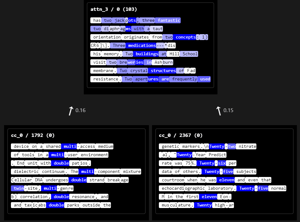
- One of the top upstream latents for attn_2 / 0 fires specifically on "of the", even though attn_2 / 0 itself fires on capitalized words following "of".attn_3 / 0 fires on mentions of two or three of an object (e.g. "three apples"). But a top upstream latent fires on "multi-", "double-", "twin-" etc, which is a related but distinct context.cc_3 / 10 fires on token(s) after a "y" token, but a top upstream latent fires on tokens after words like "digital", "visual", "real", which is unrelated.
- attn_2 / 0 has 169 upstream latents, most of which seem to fire on "of" in different contexts. My approach failed to find the single "of" direction that was relevant for this computation.
Dashboards
attn_2 / 0 Capitalized words following "of"
attn_2 / 3 Tokens following letter "m"
attn_2 / 6 Countries/states/companies in news context
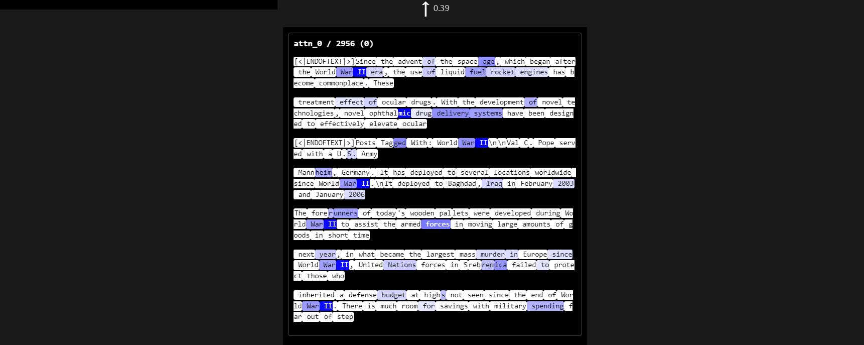
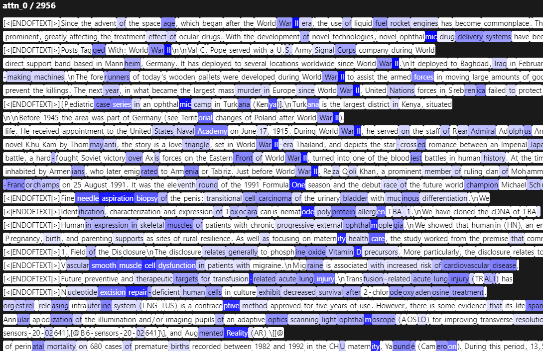
More contexts for attn_0 / 2956, which seems to fire most at the final token of a word/short phrase ("World War II", "space age", "liquid fuel", "ophthalmic")
cc_2 / 3 Biographies of notable figures, esp education section
cc_2 / 4 \n tokens in lists of (wikipedia?) categories; also "etc" token
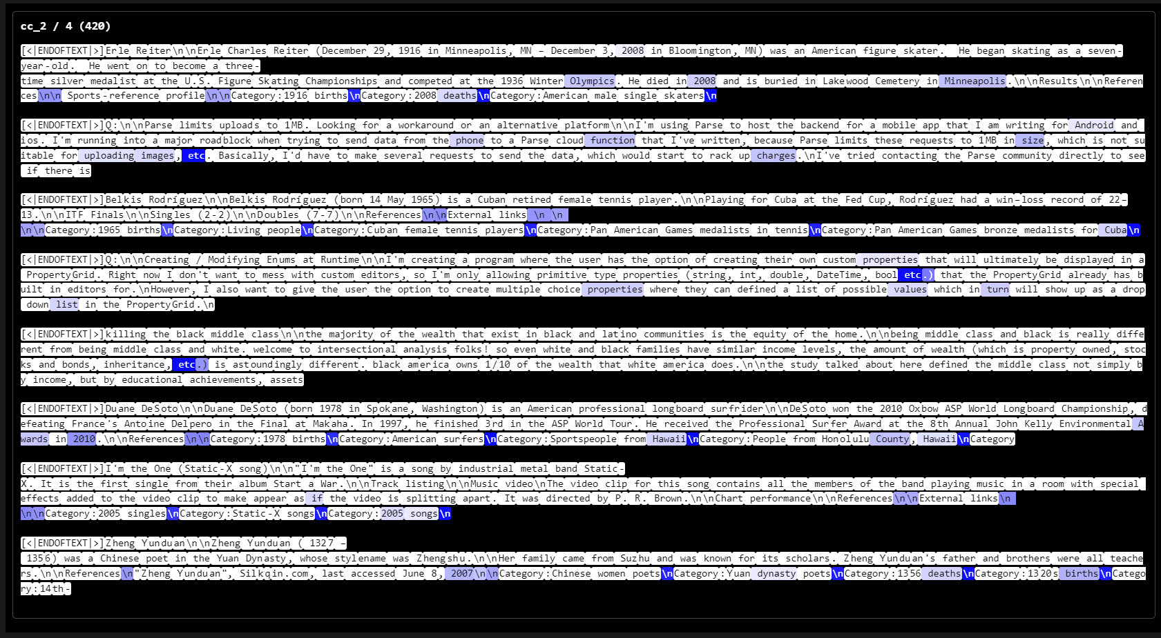
cc_2 / 6 \n inside parentheses in code, followed by spacing/indentation
attn_3 / 0 two or three objects
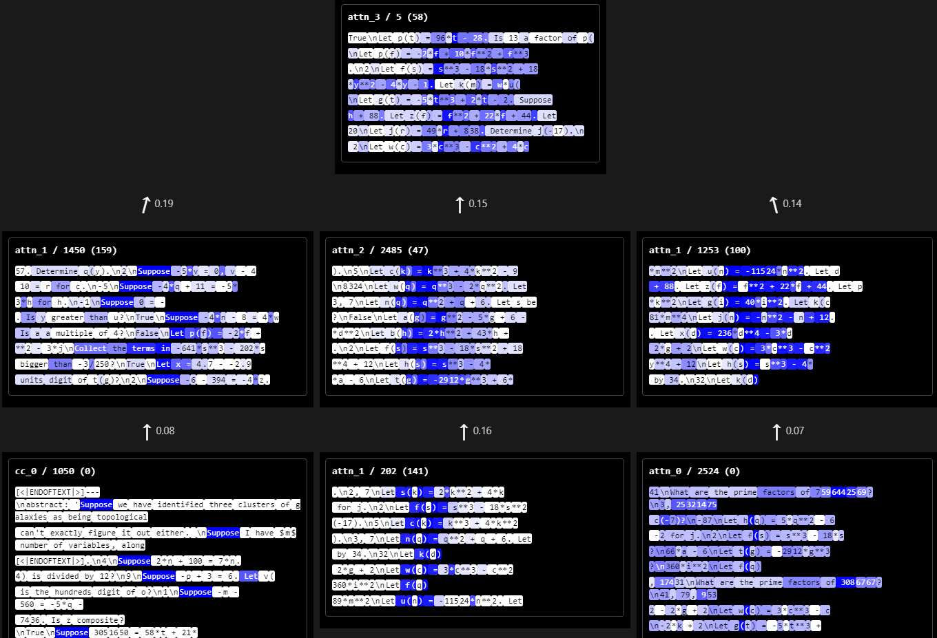
attn_3 / 5 function definitions
attn_3 / 15 repetitions/lists of things?
cc_3 / 7 polysemantic
There was no discernable pattern amongst these activations.
cc_3 / 17 token(s) after "y" token (or sometimes "w", "x", "z", and "k")
cc_3 / 24 the second of two classes of objects
How I updated on these results
This subsection is informal, and less thought-out than the rest of the post.
My main takeaway from the above results was "this all looks vaguely reasonable - I guess I finally got my code to work!". I have not updated much either way on the viability of the sparse-connectivity approach itself. The FVU Pareto curves look fine - not amazing - but what can you expect from such narrow SAEs with so many dead features? The features and connections I looked at seem fairly interpretable, but I doubt they give much more insight than taking standard SAEs and looking at the largest virtual weights[7]. In any case, I only expect obvious interpretability gains for features with <20 connections, say, rather than hundreds.
Overall, I am wary of reading much into these fairly ambiguous results when there are several practical issues to be fixed first. As mentioned before, I rushed this post out due to time constraints.
4. Limitations
Issue 1: Dead latents
Issue: Many latents die during training, likely hurting reconstruction and monosemanticity.
Fix: Use AuxK loss, or resample dead latents. Experiment with initialization, learning rate, etc.
Issue 2: High excess FVU
Issue: Excess FVU remains high even without masking.
Fix: This tells us that error accumulation hurts reconstruction. Following Marks et al (2024), we could include contributions from upstream SAE errors. However, this risks encouraging error terms to get larger so that downstream dictionaries can read off from them. A safer approach might be detaching SAE errors from the computational graph before including them.
Increasing SAE width, avoiding dead latents, and switching from TopK to BatchTopK should also help.
Issue 3: Memory
Issue: Each mask and virtual weight matrix has elements, with dictionary pairs total, where F is dictionary width and is layer count. So memory scales as , prohibiting scaling to large models.
Fix for masks: Do not use masking for the first x% of training. Then use co-occurrence statistics to identify 1000 (say) candidate connections per latent. Store soft-mask values only for these candidates, setting others to zero, and continue training with the mask as usual. This reduces memory to with a manageable constant factor.
Fix for virtual weights: Recall Eq (3) defining the sparsely-connected forward pass: . If we are content to replace with or , then the the virtual weight matrix is no longer a leaf node of the computational graph, so we don't need to store all virtual weights during a forward pass, reducing memory from to . This memory scaling may still be prohibitively expensive (though at least it does not scale with the training batch size).
Issue 4: Feature splitting
Issue: Dictionaries find many, granular features in cases where we'd prefer they find a single, computationally-relevant one. E.g. a downstream latent might have connections to an "elephant" latent and a "lizard" latent and a "cat" latent, etc, resulting in hundreds of connections when a single "animal" latent would have sufficed.
Fix: Matryoshka SAEs (Bussman & Leask; Nabeshima) have been shown to mitigate feature splitting. For future work, I suggest using Matryoshka BatchTopK SAEs. But:
The issue may be fundamental to SAEs: @Lucius Bushnaq notes that both broad ("animal") and specific ("elephant," "lizard," "cat") directions can be computationally relevant in different contexts. We therefore want dictionaries to capture both. But doing so would lead to bad reconstruction, since certain directions would be "double-counted" (see Lucius' post for a better explanation).
Possibly, my current setup can be modified to address this concern. Alternatively, one can accept the issue as annoying but not fatal. Following Anthropic, when building a feature circuit, one can group heavily-split latents into "supernodes". E.g. "elephant", "lizard" and "cat" might get grouped together into a single "animal" node. This fix does not feel ideal, but nonetheless, Anthropic has used it quite successfully.
5. Conclusion
The overall goal of this line of work is to accurately reconstruct model activations using a very small number of connections per latent, and explain more of a model's behavior (for a given size of feature circuit) than prior methods. To reach this goal, the issues outlined §4 will likely need to be fixed; until they are, it is hard to update much on the viability of the sparse-connectivity approach.
I started this project because the approach felt right to me. It makes explicit the vision of feature circuits that Anthropic seems to implicitly endorse: namely, that one feature should only depend on, and affect, a small number of others. If my approach cannot be made to work, then this intuition may need to be adjusted. Since the results in this post did not update me much, I still think the approach feels right.
Acknowledgements
Thank you to @Logan Riggs and @Jannik Brinkmann for their help near the start of this project. In particular, they encouraged the virtual weights framing, and suggested making the binary mask learnable rather than estimated at the start of training.
Thank you also to Caden Juang (@kh4dien) for a major code rewrite that led to a ~2x training speedup. He also implemented AuxK loss and multi-GPU support, which were not used in the current work but will likely be valuable in the future.
Appendix A: Prior work
The main ingredients for my work come from two papers: Anthropic (2025), which introduces CLTs, and Farnik et al (2025), which aims to sparsify connections between SAE latents. In this section, I briefly summarize the relevant parts of these papers, and explain the improvements offered by my approach.
Circuit Tracing/Circuit Biology - Anthropic (2025)
Anthropic trains CLTs at every layer. They do not use attention SAEs. To assemble latents into circuits, they compute contributions of upstream features to downstream ones on a given prompt, and build a feature circuit (aka "attribution graph") by keeping edges between latents where the contribution exceeds some threshold. Contributions can be computed exactly since attention is frozen. They do not train for sparse connectivity.
As well as prompt-dependent feature circuits, they also analyze virtual weights. They highlight some problems with interpreting virtual weights; below each quote I summarize how my work addresses the problem.
There is one major problem with interpreting virtual weights: interference. Because millions of features are interacting via the residual stream, they will all be connected, and features which never activate together on-distribution can still have (potentially large) virtual weights between them.
Virtual weights between non-coactivating latents will be masked out during training.
In some cases, the lack of activity of a feature, because it has been suppressed by other features, may be key to the model’s response... By default, our attribution graphs do not allow us to answer such questions, because they only display active features... how can we identify inactive features of interest, out of the tens of millions of inactive features?
One might think that these issues can be escaped by moving to global circuit analysis. However... we need a way to filter out interference weights, and it's tempting to do this by using co-occurrence of features. But these strategies will miss important inhibitory weights, where one feature consistently prevents another from activating.
Masking removes unimportant connections; the remaining nonzero virtual weights can be negative, i.e. inhibitory.
The basic global feature-feature weights derived from our CLT describe the direct interactions between features not mediated by any attention layers. However, there are also feature-feature weights mediated by attention heads... Our basic notion of global weights does not account for these interactions at all.
I use attention SAEs for this reason. Connections to downstream attention SAE latents pass through the OV circuit.
Jacobian SAEs - Farnik et al (2025)
Farnik et al also pursue sparse connectivity. They train two SAEs in tandem: one to reconstruct an MLP's input, and one for the output. At each update step, they compute the matrix of derivatives of output latent activations with respect to input ones (aka the Jacobian). They add the norm of to the training loss. This term encourages to be “sparse” in a weak sense: on any given token, the set of entries of has high kurtosis (as opposed to the strong sense of most entries equaling zero). That is, at linear order, an output latent has a small number of input latents contribute a large amount to it.
My approach has two main advantages:
- I produce a forward pass where each latent activation is exactly sparse in terms of upstream ones: no linear approximation is taken, and there is no long tail of small contributions from upstream latents.I sparsify an entire network, rather than just one submodule.
A further difference between our approaches: in my approach, a downstream latent gets its contributions from the same set of upstream ones, regardless of context; in Farnik et al, the set of highly-contributing upstream latents may be different on each token. My notion of sparse connectivity is therefore more constraining. (I don't claim that my notion is necessarily the "correct" one. Both seem useful.)
Appendix B: Virtual weights for downstream attention
Let be the OV matrix of the attention layer, with shape [n_heads, d_model_out, d_model_in]. Define the virtual weights , with shape [n_heads, n_latents_down, n_latentsup], as:
<span class="mjx-math" aria-label="V{hij} = \sum{\alpha,\beta}(W^u\text{dec}){j\alpha} (OV){h\beta\alpha} (W^d\text{enc}){\beta i}">
indexes head; indexes n_latents_down; indexes n_latents_up; indexes d_model_in; indexes d_modelout.
Now let <span class="mjx-math" aria-label="F^d{qi}"> be the -th downstream latent activation at sequence position .
Let be the attention probability of head in the downstream attention layer, between query position and key position .
Let be the downstream layernorm scale just before attention, at query position .
Finally, we can write our new version of Eq (2):
This equation expresses downstream latent activations as a linear combination of upstream ones, with coefficients given by virtual weights (times some attention probability and layernorm factors).T
- ^
AFAIK, feature circuit research began with Olah et al (2020), and was first applied to language models by Marks et al (2024). Please correct me if I've overlooked important prior work. Anthropic (2025) is the most recent major contribution.
- ^
Analogy taken from @Lucy Farnik's post. The section Why we care about computational sparsity motivates the current work. I was also motivated by Activation space interpretability may be doomed, plus the following off-hand remarks:
@Daniel Tan (source): If someone figures out how to train SAEs to yield sparse feature circuits that'll also be a big win.
@StefanHex (source): Interactions [between features], by default, don't seem sparse... In practice this means that one SAE feature seems to affect many many SAE features in the next layers, more than we can easily understand.
- ^
Fixing the issue should improve reconstruction and feature monosemanticity, but since I will be busy with MATS for a couple months, I'm publishing now rather than waiting for a fix.
- ^
E.g. this is true if has input (resid_pre, ) and upstream dictionaries reconstruct (attn_out, ) and (mlp_out, ) for each layer , as well as (resid_pre, 0).
- ^
i.e. "just travel along the residual stream, without applying any attention or MLP blocks".
- ^
This is a small lie. When is an attention SAE, attention probabilities will now appear somewhere on the RHS - see Eq (4) in the appendix.
- ^
Yes, I should have checked this! Unfortunately, I had to rush this post out.
Discuss
