
Published on July 9, 2024 10:06 PM GMT
Thanks to the many people I've chatted with this about over the past many months. And special thanks to Cunningham et al., Marks et al., Joseph Bloom, Trenton Bricken, Adrià Garriga-Alonso, and Johnny Lin, for crucial research artefacts and/or feedback.
Codebase: sparse_circuit_discovery
TL; DR: The residual stream in GPT-2-small, expanded with sparse autoencoders and systematically ablated, looks like the working memory of a forward pass. A few high-magnitude features causally propagate themselves through the model during inference, and these features are interpretable. We can see where in the forward pass, due to which transformer layer, those propagating features are written in and/or scrubbed out.
Introduction
What is GPT-2-small thinking about during an arbitrary forward pass?
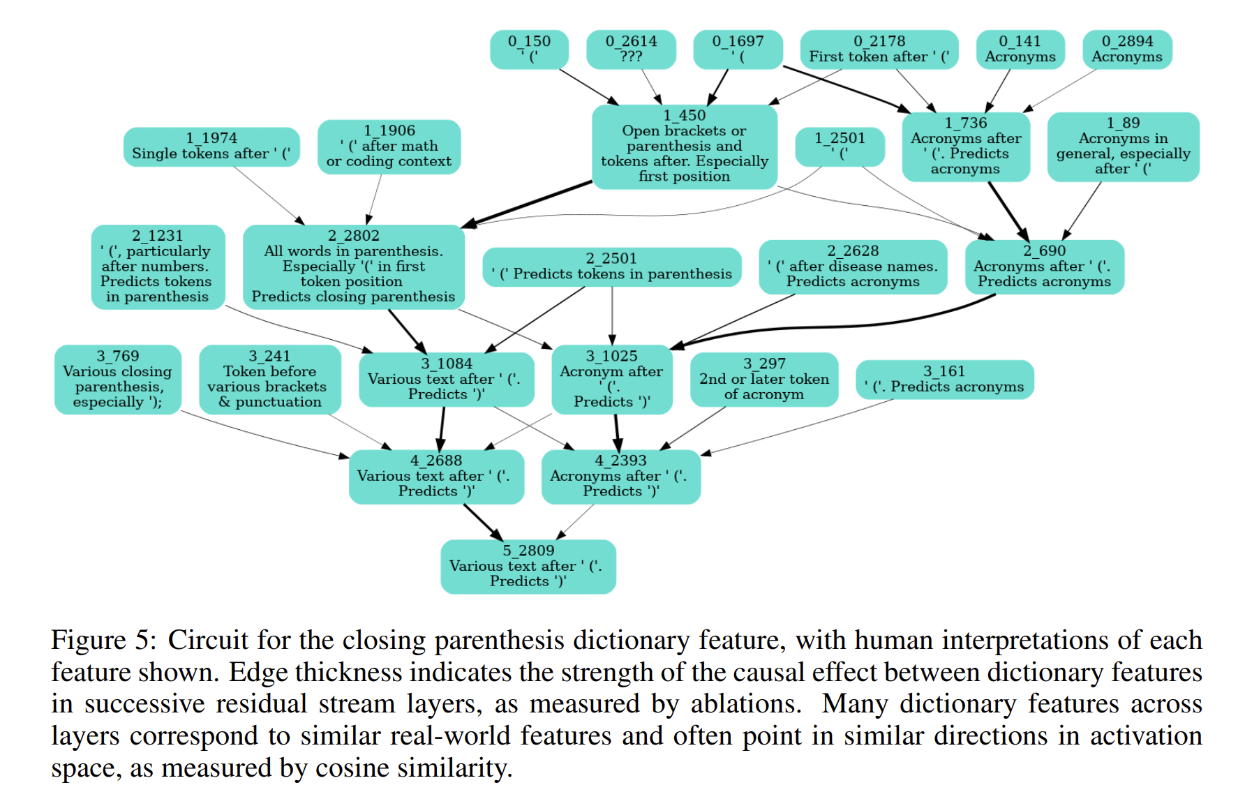
I've been trying to isolate legible model circuits using sparse autoencoders. I was inspired by the following example, from the end of Cunningham et al. (2023):
I wanted to see whether naturalistic transformers[1] are generally this interpretable as circuits under sparse autoencoding. If this level of interpretability just abounds, then high-quality LLM mindreading & mindcontrol is in hand! If not, could I show how far we are from that kind of mindreading technology?
Related Work
As mentioned, I was led into this project by Cunningham et al. (2023), which established key early results about sparse autoencoding for LLM interpretability.
While I was working on this, Marks et al. (2024) developed an algorithm approximating the same causal graphs in constant time. Their result is what would make this scalable and squelch down the iteration loop on interpreting forward passes.
Methodology
A sparse autoencoder is a linear map, whose shape is (autoencoder_dim, model_dim). I install sparse autoencoders at all of GPT-2-small's residual streams (one per model layer, in total). Each sits at a pre_resid bottleneck that all prior information in that forward pass routes through.[2]
I fix a context, and choose one forward pass of interest in that context. In every autoencoder, I go through and independently ablate out all of the dimensions in autoencoder_dim during a "corrupted" forward pass. For every corrupted forward pass with a layer sparse autoencoder dimension, I cache effects at the layer autoencoder. Every vector of cached effects can then be reduced to a set of edges in a causal graph. Each edge has a signed scalar weight and connects a node in the layer autoencoder to a node in the layer autoencoder.
I keep only the top- magnitude edges from each set of effects , where is a number of edges. Then, I keep only the set of edges that form paths with lengths .[3]
The output of that is a top- causal graph, showing largest-magnitude internal causal structure in GPT-2-small's residual stream during the forward pass you fixed.
Causal Graphs Key
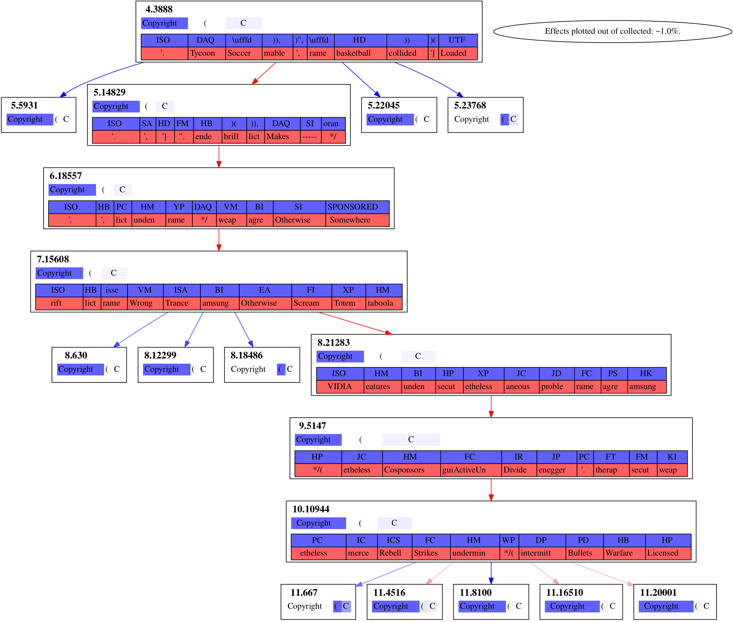
Consider the causal graph below:
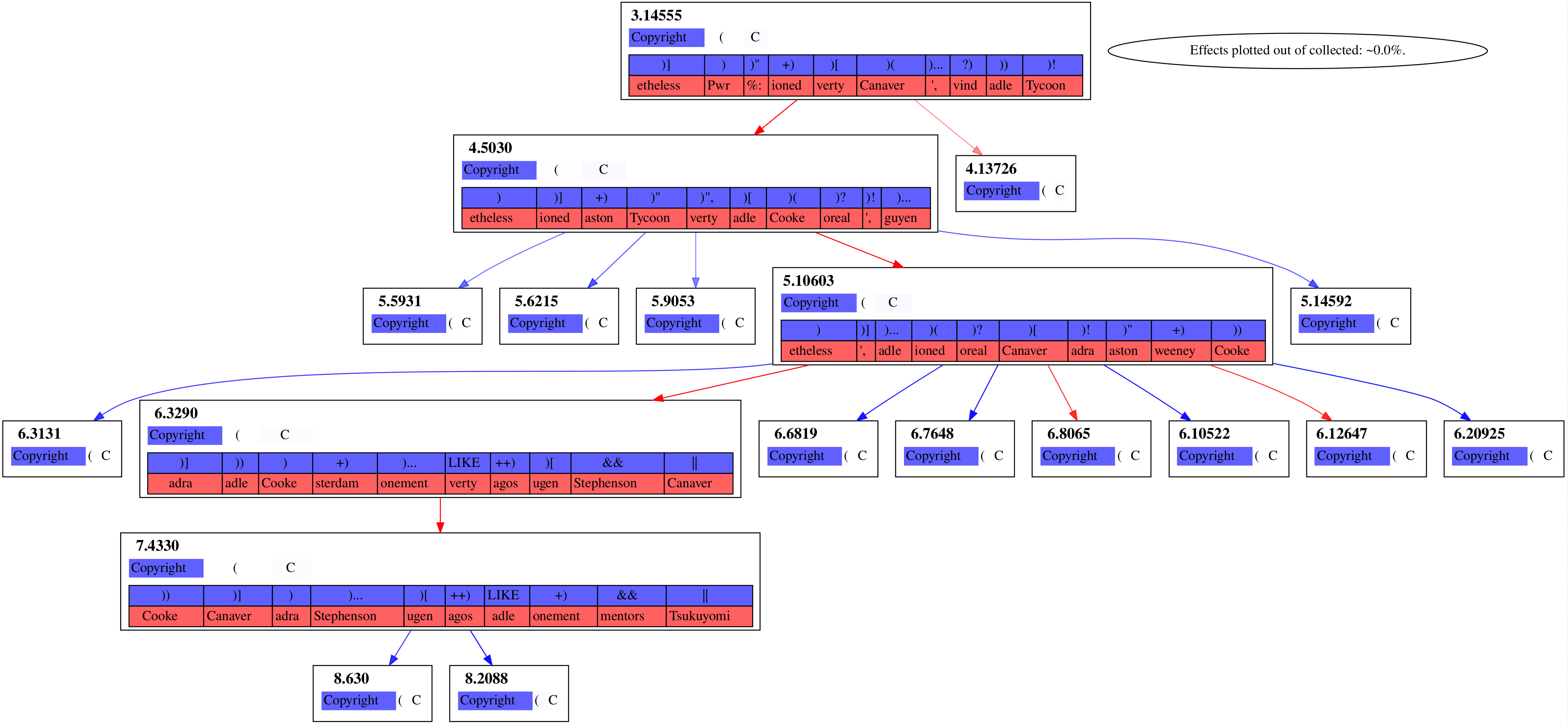
Each box with a bolded label like 5.10603 is a dimension in a sparse autoencoder. 5 is the layer number, while 10603 is its column index in that autoencoder. You can always cross-reference more comprehensive interpretability data for any given dimension on Neuronpedia using those two indices.
Below the dimension indices, the blue-to-white highlighted contexts show how strongly a dimension activated following each of the tokens in that context (bluer means stronger).
At the bottom of the box, blue or red token boxes show the tokens most promoted (blue) and most suppressed (red) by ablating that dimension.
Arrows between boxes plot the causal effects of an ablation on dimensions of the next layer's autoencoder. A red arrow means ablating dimension will also suppress downstream dimension . A blue arrow means that ablating promotes downstream dimension . Color transparency indicates effect size.
Results
Parentheses Example
Our context is Copyright (C. This tokenizes into Copyright, (, and C. We look at the last forward pass in that context.
Even GPT-2-small is quite confident as to how this context should be continued in its final forward-pass:
| Top Next Token | Probability |
|---|---|
) | 82.3% |
VS | 0.9% |
AL | 0.6% |
IR | 0.5% |
)( | 0.5% |
BD | 0.4% |
SP | 0.4% |
BN | 0.4% |
Our algorithm then yields four causal graphs out.
Figure 1
Figure 2
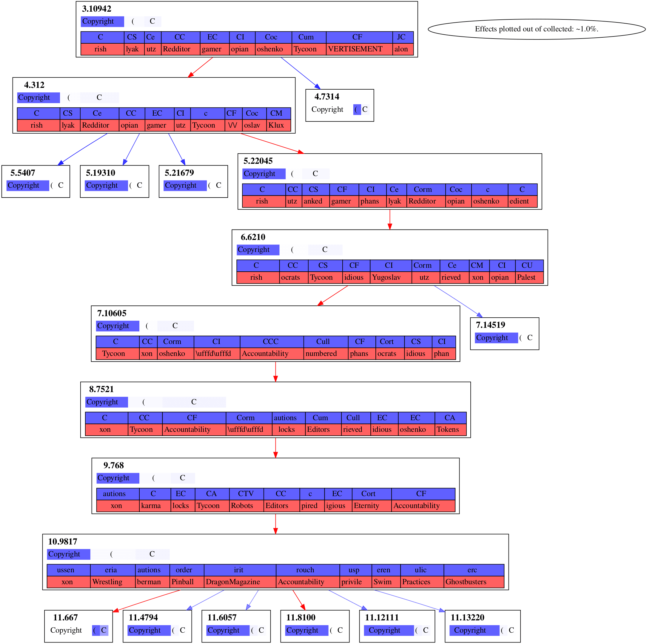
Figure 3
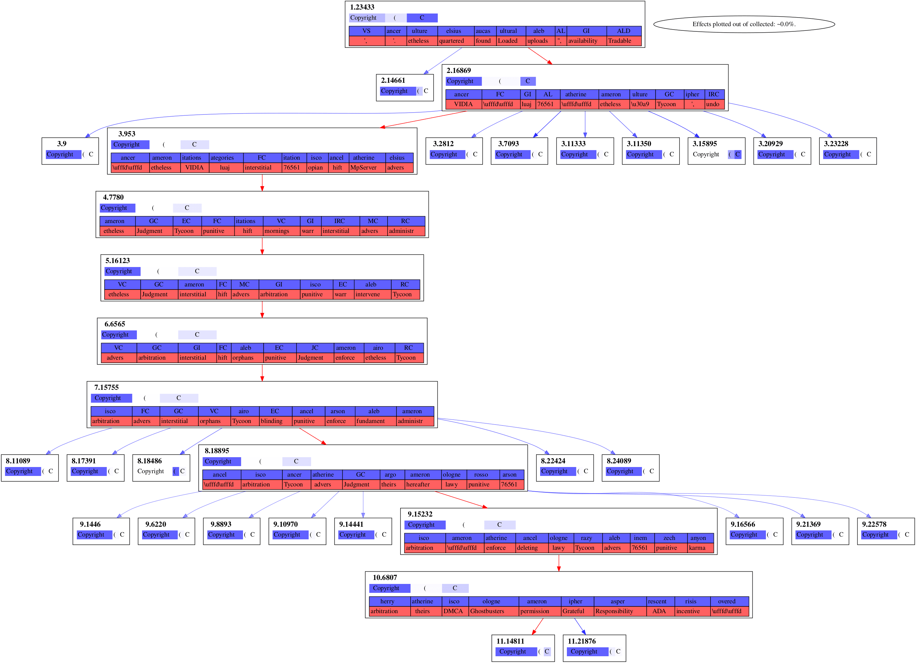
Figure 4
It's notable that these graphs of strong effects aren't connected to the embedding layer, layer . Even Figure 3, whose chain of features spans the rest of the model, isn't connecting to the embedding layer. I suspect that's due to attention layers being what's writing in these directions, rather than the embedding layer at that forward pass being what's writing it in.
Notice that dimensions 11.667 and 11.8100 are being strongly downweighted in Figure 4 while being strongly upweighted in Figure 2.
Validation of Graph Interpretations
Can we straightforwardly assess what each causal graph does by looking over its nodes and edges?
Fig. 1 - Parentheticals
The features in Figure 1 all involve being inside parentheticals. Let's see what Figure 1 does in another context where GPT-2-small will still complete a close parentheses after an open parentheses. If we prompt with "In a Lisp dialect, every expression begins with ( and ends with", the model's final sequence position logits are:
| Top Next Token | Probability |
|---|---|
) | 42.2% |
). | 14.9% |
), | 4.8% |
. | 3.8% |
, | 3.0% |
a | 1.8% |
; | 1.8% |
( | 1.7% |
Ablating out the parentheticals causal path in this context has the following effects:
| Top Upweighted Next Token | Probability Difference | Top Downweighted Next Token | Probability Difference[4] |
|---|---|---|---|
( | +32.6% | ) | -42.2% |
a | +6.5% | ). | -14.9% |
the | +4.0% | ), | -4.8% |
\n | +1.4% | , | -1.7% |
an | +1.2% | .) | -1.5% |
and | +0.6% | ); | -1.0% |
$ | +0.5% | ; | -1.0% |
. | +0.4% | ): | -0.6% |
Fig. 2 - C-words
We can similarly check the other subgraphs, just prompting with something matching their interpretation. For Figure 2, which on its face deals with C-words,
"<|endoftext|>According to a new report from C"
| Top Next Token | Probability |
|---|---|
NET | 14.9% |
iti | 10.4% |
rain | 6.1% |
- | 3.6% |
og | 3.0% |
Net | 2.8% |
IO | 2.4% |
Q | 2.0% |
| Top Upweighted Next Token | Probability Difference | Top Downweighted Next Token | Probability Difference[5] |
|---|---|---|---|
. | +29.2% | NET | -14.9% |
, | +6.1% | iti | -10.4% |
- | +3.0% | rain | -6.1% |
that | +2.2% | og | -3.0% |
ratings | +2.2% | Net | -2.8% |
the | +1.0% | IO | -2.4% |
early | +1.0% | Q | -2.0% |
and | +1.0% | TV | -1.6% |
Fig. 3 - C-words
Same context as last, with identical base probabilities.
| Top Upweighted Next Token | Probability Difference | Top Downweighted Next Token | Probability Difference[6] |
|---|---|---|---|
ri | +7.2% | NET | -14.9% |
rain | +5.2% | iti | -4.9% |
uy | +4.4% | Net | -2.7% |
- | +3.4% | IO | -2.4% |
iner | +2,2% | Q | -1.5% |
att | +2.1% | ME | -1.2% |
og | +2.0% | TV | -0.9% |
rav | +1.8% | NA | -0.9% |
Fig. 4 - Acronyms
"<|endoftext|>Foreign Direct Investment (F"
| Top Next Token | Probability |
|---|---|
DI | 99.9% |
D | 0.0% |
DR | 0.0% |
ID | 0.0% |
DD | 0.0% |
DE | 0.0% |
DF | 0.0% |
ED | 0.0% |
| Top Upweighted Next Token | Probability Difference | Top Downweighted Next Token | Probability Difference[7] |
|---|---|---|---|
irms | +19.4% | DI | -80.7% |
ulf | +2.9% | DE | -0.0% |
int | +2.4% | ||
ares | +2.4% | ||
acing | +2.3% | ||
aced | +2.2% | ||
annie | +1.9% | ||
ailing | +1.4% |
Other Validation
Ablating out every autoencoder dimension except the ones in question turned out to be too destructive, and just makes a hash of the output logits. That is too far out of distribution, apparently, and so the strongest possible form of the causal-graphs-as-circuits hypothesis here must be false.
Ablating during randomly sampled openwebtext forward-passes yields basically random effects. This fits with circuit activation being quite contextual. But it's disappointing, again, that we don't see no effect whatsoever on off-distribution contexts.
All in all, I wish I lived in a world with that stronger validation data. I am very open to other suggestions as to how to stress-test interpretations of causal graphs!
Discussion
"The Residual Stream Is Working Memory..."
People often say that each transformer block reads/writes to the residual stream. This statement, I think, is a way of thinking about the architecture. It's a stronger hypothesis to say that what's in the residual stream is straightforwardly interpretable.
What I think is going on here is that the business logic of the learned program in the transformer is separated into different software modules. Each transformer block is one software module. Those modules read and write from the residual stream, and use that stream as a scratchpad to represent the running hypothesis for next token.
"...And It Is Easily Interpretable."
And, we can just see where in the forward pass a hypothesis about the next token comes into existence! If that hypothesis is scrubbed out, we can see where that happens too. We can see what layer is causally responsible for those operations. In essence, interpreting the residual stream in this way gives the "what" and "where" of transformer cognition: we see what is represented across the residual stream. If anything in the residual stream is then of interest, we just then have to understand the causally originating transformer block to get the relevant "how."
Conclusion
When you look at the effects of sparse-autoencoder ablations in GPT-2-small during inference, in the residual stream, you see a few causal paths from autoencoder dimension to autoencoder dimension. These causal paths seem to all deal in one meaning. Specifically, in the context "Copyright (C", you see causal paths for C-words, for parentheticals, and for acronyms in the final forward-pass.
- ^
I.e., transformers trained on real-world data, as opposed to toy data.
- ^
Ablation Hook Structure
def ablate_hook_fac( dim_indices: list[int], encoder: t.Tensor, enc_biases: t.Tensor, decoder, dec_biases, ): """Create hooks that zero projected neurons and project them back.""" def ablate_hook( # pylint: disable=unused-argument, redefined-builtin module, input, output ) -> None: """ Project activation vectors; ablate them; project them back. """ # Project through the encoder. Bias usage now corresponds to Joseph # Bloom's (and, by way of him, Antropic's). projected_acts = ( t.nn.functional.linear( # pylint: disable=not-callable output[0] - dec_biases.to(model.device), encoder.T.to(model.device), bias=enc_biases.to(model.device), ) ).to(model.device) t.nn.functional.relu( projected_acts, inplace=True, ) # Zero out or otherwise pin the column vectors specified. mask = t.ones(projected_acts.shape, dtype=t.bool).to(model.device) if coefficient == 0.0: mask[:, :, dim_indices] = False else: mask = mask.float() mask[:, :, dim_indices] = coefficient ablated_acts = projected_acts mask projected_acts = ( t.nn.functional.linear( # pylint: disable=not-callable projected_acts, decoder.T.to(model.device), bias=dec_biases.to(model.device), ) ) ablated_acts = ( t.nn.functional.linear( # pylint: disable=not-callable ablated_acts, decoder.T.to(model.device), bias=dec_biases.to(model.device), ) ) # Perform the ablation. The right term reflects just ablation # effects, hopefully canceling out autoencoder mangling. We must # also preserve the attention data inoutput[1]. return ( output[0] + (ablated_acts - projected_acts), output[1], ) return ablate_hook - ^
Other details:
- All ablations are zero-ablations.Ablation effects are the difference between corrupted and unaltered forward passes, at the layer autoencoder.Runtime and memory are both in , being
autoencoder_dim. - ^
Ablating out a control causal path with equal placement and dimension count
3: [0]4: [0]5: [0]6: [0]7: [0]instead gives effects
Top Upweighted Next Token Probability Difference Top Downweighted Next Token Probability Difference .+3.4% )-3.0% ,+1.6% ).-2.3% ):+0.5% .)-1.2% \n+0.5% ),-0.9% );+0.5% (-0.4% )+0.4% ---0.3% :+0.4% --0.3% ).+0.4% ++-0.2% - ^
3: [0]4: [0]5: [0]6: [0]7: [0]8: [0]9: [0]Top Upweighted Next Token Probability Difference Top Downweighted Next Token Probability Difference Q+7.9% NET-14.8% red+5.4% rain-4.9% AG+5.2% --2.9% ough+3.2% Net-2.7% FO+2.7% iti-1.9% &+2.2% IO-1.6% GA+1.7% TV-1.5% RS+1.5% NA-0.9% - ^
1: [0]2: [0]3: [0]4: [0]5: [0]6: [0]7: [0]8: [0]9: [0]10: [0]Top Upweighted Next Token Probability Difference Top Downweighted Next Token Probability Difference AG+11.9% NET-14.9% ough+5.4% iti-6.2% Q+5.1% rain-5.7% red+4.2% --3.0% MA+3.2% Net-2.7% uts+3.0% IO-2.1% &+2.8% TV-1.6% ut+1.6% oint-0.9% - ^
4: [0]5: [0]6: [0]7: [0]8: [0]9: [0]10: [0]Top Upweighted Next Token Probability Difference Top Downweighted Next Token Probability Difference DF+0.6% DI-1.5% OD+0.2% IDE-0.0% ID+0.2% dn-0.0% D+0.1% ined-0.0% DD+0.0% di-0.0% DE+0.0% DIT-0.0% DT+0.0% ido-0.0% DO+0.0% ded-0.0% - ^
Spot-Check Other Multiplicative Coefficients
Can we assume that a full zero-ablation implies much about causal effects in other, milder cases?
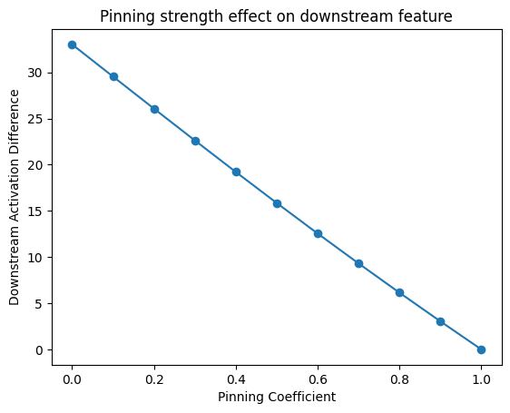
Here are the effects of other multiplicative coefficients besides , scaling dimension
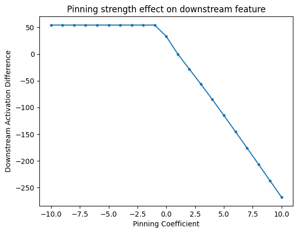
3.953, on the downstream dimension4.7780.Here's the graph again with an order-of-magnitude wider coefficient grain:
The response here is almost linear—there is a single discontinuity.
Discuss
