该研究探讨了神经网络在叠加状态下计算新特征的机制，并提出了一个假设：神经网络需要某种形式的错误校正来避免干扰失控。研究通过两个实验验证了这一假设：激活平台实验和敏感方向实验。结果表明，真实激活在受到微小扰动时表现出平台效应，即扰动对模型输出的影响小于预期。此外，将真实激活扰动至另一个真实激活的方向上，比扰动至随机方向上更容易影响模型输出。

🤔 **激活平台实验：** 该实验旨在验证神经网络是否具有错误校正机制，以抑制特征激活中的微小噪声。实验结果显示，真实激活在受到随机方向扰动时，其模型输出的变化小于随机激活。这表明，真实激活位于一个平台的中心，即在一定范围内，扰动对模型输出的影响很小。

🧭 **敏感方向实验：** 该实验进一步验证了神经网络的错误校正机制。实验结果表明，将真实激活扰动至另一个真实激活的方向上，其模型输出的变化比扰动至随机方向上更快。这说明，真实激活方向比随机方向更加敏感，即更容易受到扰动影响。

💡 **稀疏自动编码器（SAE）与模型行为：** 研究人员提出了一个假设：SAE特征与叠加计算模型中的特征具有相同的错误校正属性。为了验证这一假设，他们计划进行以下实验： 1. 验证SAE特征是否也表现出平台效应，即在受到扰动时，其模型输出的变化小于预期。 2. 验证将真实激活扰动至SAE特征方向上，是否与扰动至另一个真实激活方向上具有类似的效果。

🤔 **SAE特征的潜在问题：** 研究人员指出，SAE特征可能存在一个潜在问题，即它们可能仅仅反映了训练数据集的特性，而不是模型内部计算的真实情况。因此，他们希望找到一种更便宜或更有效的方法来识别模型特征，而不依赖于昂贵的SAE训练过程。

🚀 **未来研究方向：** 研究人员计划进一步研究SAE特征的性质，例如： 1. SAE特征是否与叠加计算模型中的特征一致？ 2. 是否存在不同类型的SAE特征，例如原子特征和复合特征？ 3. 线性特征组合如何影响模型行为？

Published on July 5, 2024 5:05 PM GMT

This part-report / part-proposal describes ongoing research, but I'd like to share early results for feedback. I am especially interested in any comment finding mistakes or trivial explanations for these results. I will work on this proposal with a LASR Labs team over the next 3 months. If you are working (or want to work) on something similar I would love to chat!
Experiments and write-up by Stefan, with substantial inspiration and advice from Jake (who doesn’t necessarily endorse every sloppy statement I write). Work produced at Apollo Research.

TL,DR: Toy models of how neural networks compute new features in superposition seem to imply that neural networks that utilize superposition require some form of error correction to avoid interference spiraling out of control. This means small variations along a feature direction shouldn't affect model outputs, which I can test:

Activation plateaus: Real activations should be resistant to small perturbations. There should be a "plateau" in the output as a function of perturbation size.Sensitive directions: Perturbations towards the direction of a feature should change the model output earlier (at a lower perturbation size) than perturbations into a random direction.

I find that both of these predictions hold; the latter when I operationalize "feature" as the difference between two real model activations. As next steps we are planning to

Test both predictions for SAE features: We have some evidence for the latter by Gurnee (2024) and Lindsey (2024).Are there different types of SAE features, atomic and composite features? Can we get a handle on the total number of features?If sensitivity-features line up with SAE features, can we find or improve SAE feature directions by finding local optima in sensitivity (similar to how Mack & Turner (2024) find steering vectors)?

My motivation for this project is to get data on computation in superposition, and to get dataset-independent evidence for (SAE-)features.

Core results & discussion

I run two different experiments that test the error correction hypothesis:

Activation Plateaus: A real activation is the center of a plateau, in the sense that perturbing the activation affects the model output less than expected. Concretely: applying random-direction perturbations to an activation generated from a random openwebtext input (“real activation”) has less effect than applying the same perturbations to a random activation (generated from a Normal distribution). This effect on the model can be measured in KL divergence of logits (shown below) but also L2 difference or cosine similarity of late-layer activations.



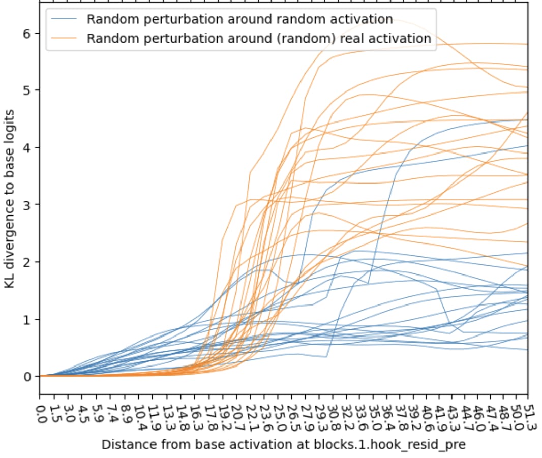
Sensitive directions: Perturbing a (real) activation into a direction towards another real activation (“poor man’s feature directions”) affects the model-outputs more than perturbing the same activation into a random direction. In the plot below focus on the size of the “plateau” in the left-hand side



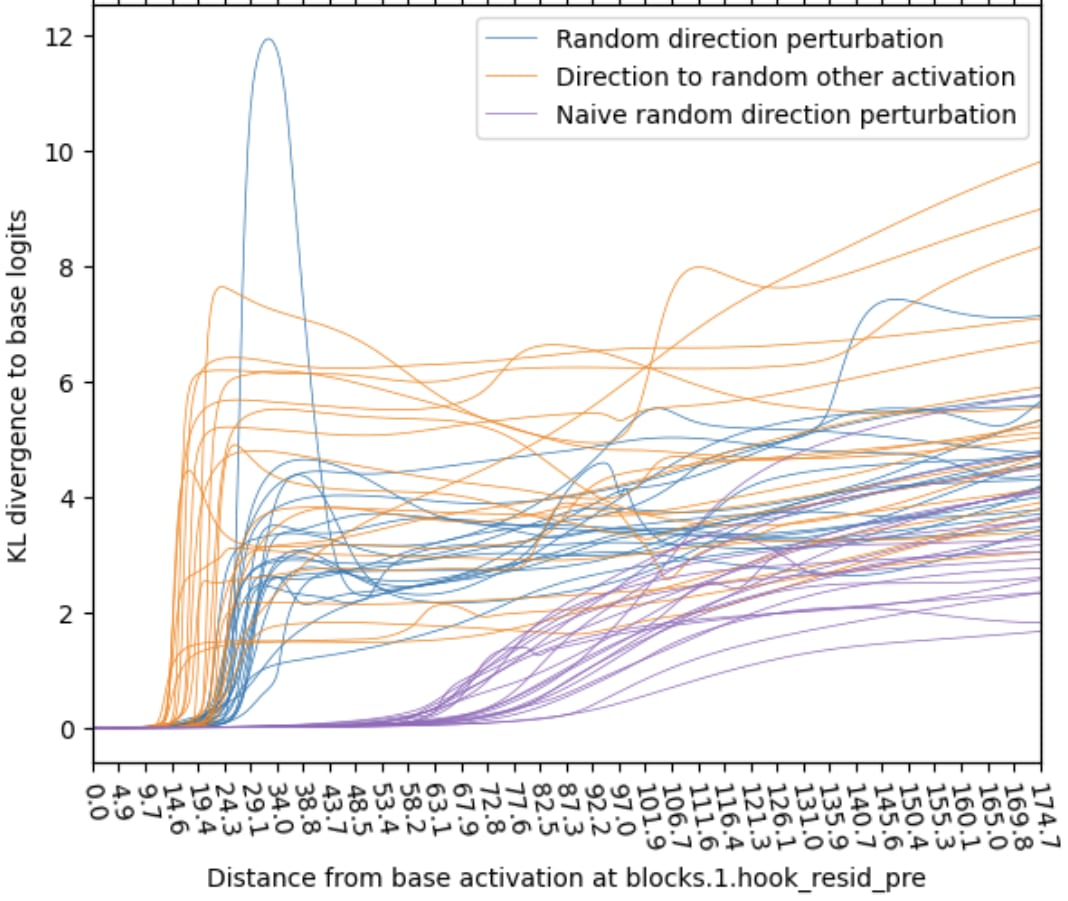
Naive random direction vs mean & covariance-adjusted random: Naive isotropic random directions are much less sensitive. Thus we use mean & covariance-adjusted random activations everywhere else in this report.The sensitive direction results are related to Gurnee (2024, SAE-replacement-error direction vs naive random direction) and Lindsey (2024, Anthropic April Updates, SAE-feature direction vs naive random direction).

The theoretical explanation for activation plateaus & sensitive direction may be error correction (also referred to as noise suppression):

NNs in superposition should expect small amounts of noise in feature activations due to interference. (The exact properties depend on how computation happens in superposition, this toy model shows one possibility.) Thus we expect NNs to have mechanisms for suppressing this noise (e.g. the “error correction” described here).Activation plateau explanation: a real activation consists of only a small number of features (on the order of L0 ~ 100) while most features (on the order of d_dictionary ~ 20k) are off. Then a random perturbation mostly induces small amounts of noise distributed over many^[1] features and causes little change in the model.Sensitive directions explanation: Perturbing a real activation creates a plateau. Its size should correspond to the perturbation size required to pass an error correction threshold in feature activations. Because perturbing towards a real other activation (“real-other”) concentrates the change in a small number of features (compared to random), we expect real-other perturbations to cross the threshold earlier, which is what we see.^[2]

Proposal: Connecting SAEs to model behaviour

The leading theory for how concepts are represented in neural networks in superposition: We think that NNs represent information as a series of sparsely-active features, which are represented as directions in activation space.^[3] Superposition allows this list of features to be much larger than the dimension of activation space, and has been demonstrated in toy models.

Sparse autoencoders (SAEs) are a method that can recover individual features from a dataset of features in superposition. SAEs are trained to convert activations into a list of sparsely-active individual features and back into activations with low reconstruction loss and high feature-sparsity. The training input for SAEs are model activations, typically generated by running the model on a dataset similar to its training data.

If SAE-features are features in the sense that computation in superposition toy models suggest, then they should show the same error correction properties we saw with real feature directions. Thus we predict

Activation Plateaus: There should also be plateaus around “artificial real” activations, created by adding & subtracting a couple of SAE features from real activations. This would confirm that activations created by shuffling around active SAE features still have the properties of real activations.Perturbing into SAE feature directions should have a similar effect as perturbing towards real-other directions (SAE features being more sensitive than random was already observed by Lindsey (2024, Anthropic April Updates) so I expect this to work). Our guess is that perturbing into single SAE directions is more sensitive (exits the plateau earlier) than spreading perturbation over multiple SAE features.

Why do I think this is a useful direction to study SAEs?

There are weird effects around how SAE features affect model behavior that we don't fully understand. Let's figure out what is going on and what we can learn!A (neglected?) failure mode of the SAE agenda is that SAE features could be an interpretability illusion in the sense that they do not represent the internal computation of the model but properties of the training dataset.
I worry that SAEs find a feature only because a concept is frequent in the dataset rather than because the model uses the concept. (I discuss this in detail in a shortform post). A dataset-independent way to find/confirm SAE features (even if non-competitive) would be great!
I’d like to find a cheaper or more targeted way to find (some or all) model features.
Training SAEs is expensive, and cost trades off against feature completeness. If we could take an individual prompt and find (all?) active features, this would be extremely useful for evaluations and interpretability research.

Conclusion

Summary: I run some experiments testing computation-in-superposition predictions on GPT2 activations, finding

Plateaus around model activations, as if the model was error-correcting small perturbationsPerturbing activations into the direction of other activations has more effect than random

I hope this research will allow us to understand computation in superposition better, and to connect behavioral properties of model activations to (SAE-)features.

Limitations: There may just be trivial explanations for results like these! Section 1 results really just say “GPT2 is weird if you go off distribution” (and happen to align with a theory prediction), but there could be lots of plausible explanations for this. Section 2 results are more specific, but still there might be simple explanations for this behavior (e.g. relevant properties of activation space beyond the covariance thing we noticed), and I would love to hear takes in the comments!

Future work: We are currently investigating these behavior properties for SAE-features, questions like

Do SAE features behave as predicted by Toy Models of Computation in Superposition?Are there different types of SAE features? Atomic and composite features?How do linear combinations of features behave? Does this give us a handle on the total number of features?

Call to action: This direction feels underexplored, I think there’s a lot of new data to be generated here! I’d love to hear from anyone considering working on this!

I also want to encourage feedback in the comments: Trivial explanations I missed? Past literature that explored this? Reasons why this direction might be less promising than I think?

Acknowledgements: We thank Dan Braun, Lee Sharkey, Lucius Bushnaq, Marius Hobbhahn, Nix Goldowsky-Dill, and the whole Apollo team for feedback and discussions of these results. We thank Wes Gurnee and Rudolf Laine for comments on a previous (March 2024) report on this project.

Appendix

Methodology

The experiments in this report focus around perturbing the residual stream of a model (via activation patching) and measuring the corresponding chance in model outputs (KL divergence and more).

All experiments use GPT2-small. Input are 10-token sequences taken from openwebtext (apollo-research/Skylion007-openwebtext-tokenizer-gpt2). We choose an early perturbation layer (blocks.1.hook_resid_pre). We read the results off at the logits (KL divergence of logprobs) or at a late layer (L2 difference of activations at blocks.11.hook_resid_post or ln_final.hook_normalized). We use only the last position index for perturbation and read-off.

Generating activations: We use model activations to measure activation plateaus, and to generate the perturbation directions for sensitivity tests. We consider 4 types of activations

Base activations: The activations of the model without any perturbation. We store the base activations at the perturbation layer and readoff layer.Random other activations (real-other): Activations on an unrelated input. We sample the perturbation layer activations corresponding to multiple (unrelated) input sequences.Random activations (random): Activation vectors generated from a multivariate normal distribution. By default I use the mean and covariance of actual activations to create slightly more realistic random activations (random), but I also test isotropic random activations (naive random). It turns out there is a big difference between naive random and sampling with the correct covariance.[SAE-feature-adjusted activations: Take the base activations but add or remove some SAE features. This is to test whether adding and removing SAE features yields activations that behave similarly to normal (real-other) activations. Not yet used in this report.]

All activation vectors have zero layer-mean (each activation has zero mean along the hidden dimension), but not zero dataset-mean (i.e. I mean-center in the same way as TransformerLens but the activation dataset mean is not the zero vector). I don’t fix the norm of activation vectors (yet).

Generating directions: In which direction to perturb the activations into. In most cases we generate an activation according to the list above and take the difference between it and the base activations to obtain a direction.

Random directions (random): Generate a random activation point (with appropriate mean and covariance) and take the difference between it and the base activations. These directions are used for the activation plateau test.Towards other activations (real-other): Sample an unrelated real activation (real-other) and take the difference between it and the base activation.[SAE decoder directions: Sample a random SAE feature (either among the currently-active SAE features, or all features). Use the corresponding decoder matrix direction (we don’t calculate a difference in this case). I test perturbation parallel (exciting the feature) or antiparallel (dampening or negatively exciting the feature) to this direction. Not yet used in this report.]

The real-other direction is a proxy for getting feature directions without having to rely on SAEs. The difference between two real activations should be a couple hundred features (about half of them negative) because each real activation should consist of a number (~L0) of features.

Perturbations: I perturb the base activation by adding αdirection to the activation vector. I do this in two ways:

Straight mode: Scale the direction such that norm(direction) = norm(base activation) and scan from α = 0 to 1.Sphere mode: Move along the sphere of constant norm (slerp) from the base activation towards the direction, all the way to its antipode. The direction just determines which “meridian” to move along, the perturbation size is measured by the angle between base activation and perturbed activation θ = 0° to 180°.

Effect on model outputs: To measure the effectiveness of a perturbation I measure the KL divergence between the perturbed model output logits and the base output logits, the L2 difference and cosine similarity between the activations in a late layer taken on the base and perturbed runs.

Experiment types: I run three types of experiments. In all cases I measure the effect of activation perturbations (as a function of perturbation L2 distance α or angle θ) on model outputs (KL divergence, final-layer L2 distance).

Activation plateaus: Starting from either a random or real activation we perturb into a random direction. In essence, we measure the existence of plateaus around different activations.Sensitive directions: Starting from a real activation we perturb into either a random or real-other direction. In essence, we measure the plateau size in different directions.Sensitivity-optima: Starting from a real activation we perturb into a 2d manifold of directions. We find the set of directions by three-way interpolating between two random directions and a real-other direction. For each interpolated direction we report the size of the plateau, measured by the distance required to have a KL divergence of >0.5 in the output. We test whether the real-other direction is a local optimum in the meta-landscape of directions.
The sensitive direction test finds the distance (α) or angle (θ) required for a certain amount of change in outputs (KL divergence of 0.5). We repeat the test for many nearby directions, and see whether the original real-other direction is a local optimum of sensitivity (α or θ).The goal of this is to find out whether real-other directions could be found by optimizing sensitivity over directions.

Detailed results

1. Activation Plateaus

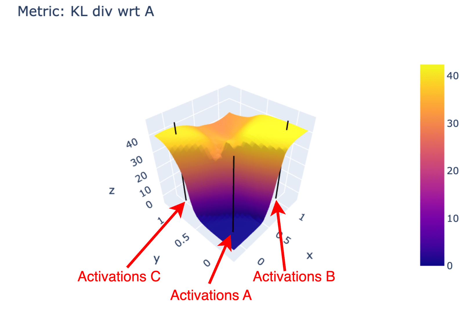
Intuition: Look at the model-output landscape when interpolating activations on the plane spanned by three real activations. The plot below shows the KL divergence (wrongly normalized, z-axis and color) for all activations on that plane. We see plateaus around the real activations (black vertical lines) with outputs changing less per shift in activations. This gives an intuitive picture; for the quantitative study we switch to a 1D version and switch from interpolation to perturbation into random directions.

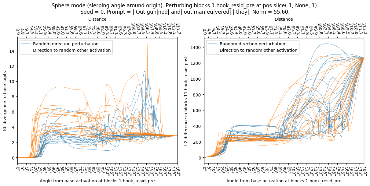
We sample a series of base activations (random or real-other) and perturb the activations from there towards a series of random directions (as discussed above we either perturb in Straight or Sphere modes). Below we show the KL div as a function of perturbation angle (Sphere case) for both types. The real-other activations clearly exhibit the plateau phenomenon—the KL div barely changes until the perturbation reaches 40°—while random activations do not follow this pattern.

Straight mode (perturbing straight into a direction):

Sphere mode (perturbing while keeping norm constant – the change between this and the plot above is due to straight/sphere mode, the seed does not have a big effect):

2. Sensitive directions

Now we perturb a given (real) base activation into different kinds of directions. This is different from the previous experiment where we applied the same (random) perturbation to different base activations.

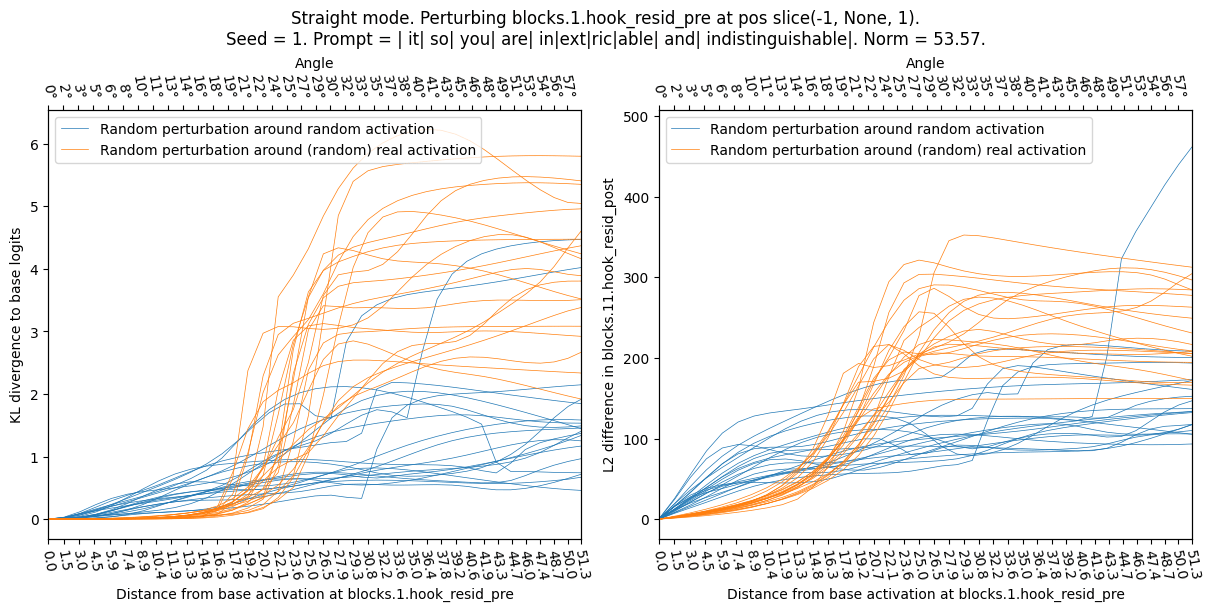
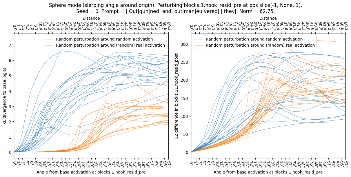
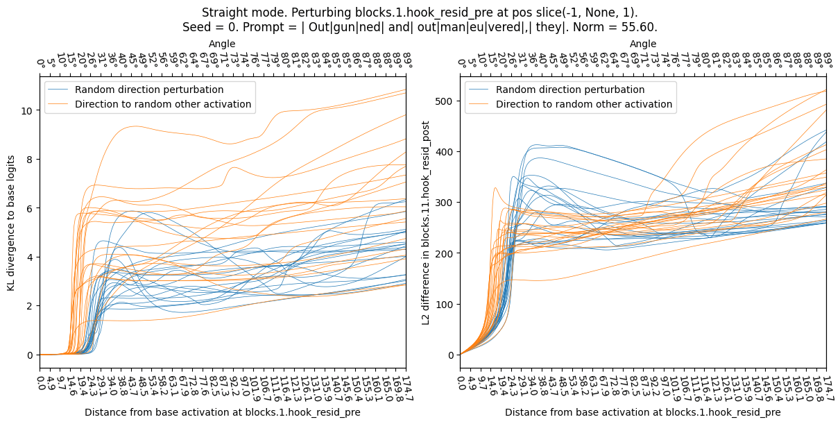
I take a given real base activation (seed / prompt shown in plot titles) and perturb it into a random direction (sample a random other activations with appropriate covariance matrix, and define direction as difference between new activation and base activation) or real-other (sample new activation by running random openwebtext sequence through model, then take difference as direction). I normalize the directions to have the same norm, and observe the effect on the model (KL div) as a function of angle (Sphere mode) or perturbation size (Straight mode). In all cases the real-other directions appear to be more sensitive, jumping up at a lower angle and lower perturbation distance.

Straight mode (perturbing straight into a direction):

Sphere mode (perturbing while keeping norm constant):

Other seeds (base prompts) looked qualitatively similar.

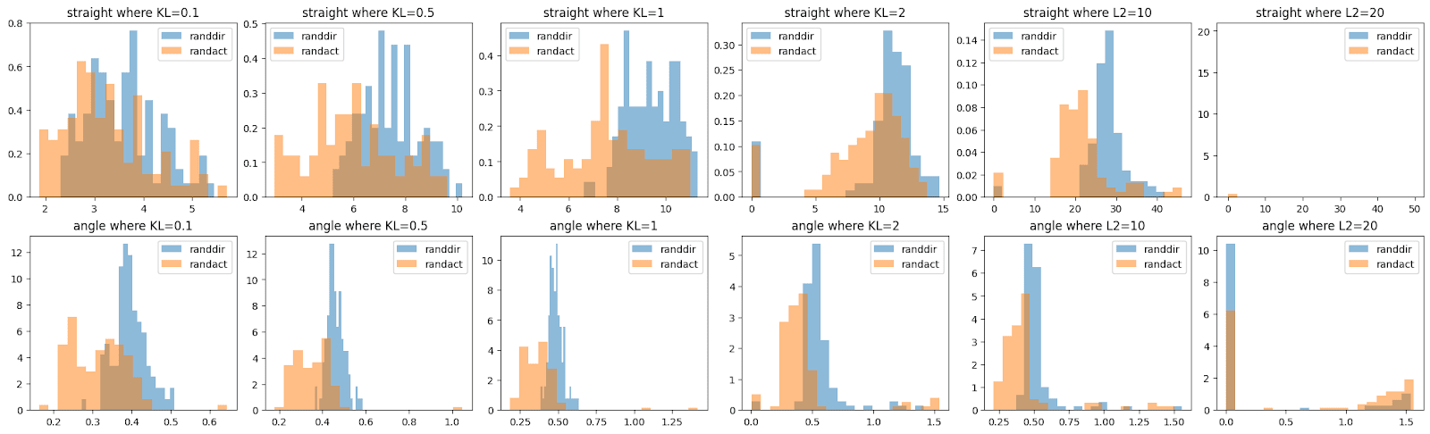
A brief investigation shows that we can find metrics, such as “at what angle does the KL divergence exceed 0.5” to reasonably distinguish the two classes of perturbation, though I think that the curves above look more distinguishable than suggested by the histograms below. (This may be an optical illusion, or show that I haven’t spent time finding the optimal classifier.)

3. Local optima in sensitivity

real-other directions are more sensitive than random directions. We think this is because they focus perturbations into a small (~L0) number of feature directions, reaching the hypothetical error correction threshold earlier.

We conjecture that, if we could perturb activations into a single feature direction, the perturbation would be even more focused and reach the error correction earlier (concretely: the perturbation distance required to reach KL-div=0.5 would be lower). This is compatible with Lindsey (2024)’s observations that SAE directions are unusually sensitive (though they did not compare to real-other or combinations of SAE directions). If that was true, we might be able to find SAE directions as local maxima of sensitivity: A perturbation into 1feature direction should be more sensitive than a perturbation into 0.99*feature direction + some other direction.

As a precursor to this investigation we investigate the sensitivity of various directions between real-other and random directions. In the plot below, every corner corresponds to a random direction (except for the top corners in the 2nd row, these correspond to real-other directions). And the color corresponds to the perturbation size (measured in Sphere mode, as angle) required to reach 0.5 KL divergence (so every point corresponds to a direction, and we run a scan over perturbation lengths on every point). The non-corner points correspond to interpolated directions (precisely: we interpolate the targets before calculating the direction). This shows us whether “nearby” directions are similarly precise as the exact real-other direction.

The upper row is a sanity-check, interpolating between 3 random directions. We expect the plot to be symmetric. The lower row is an interpolation between a real-other direction (top) and two random directions (bottom corners). We see, as expected, the top corner appears to be a local optimum of sensitivity:

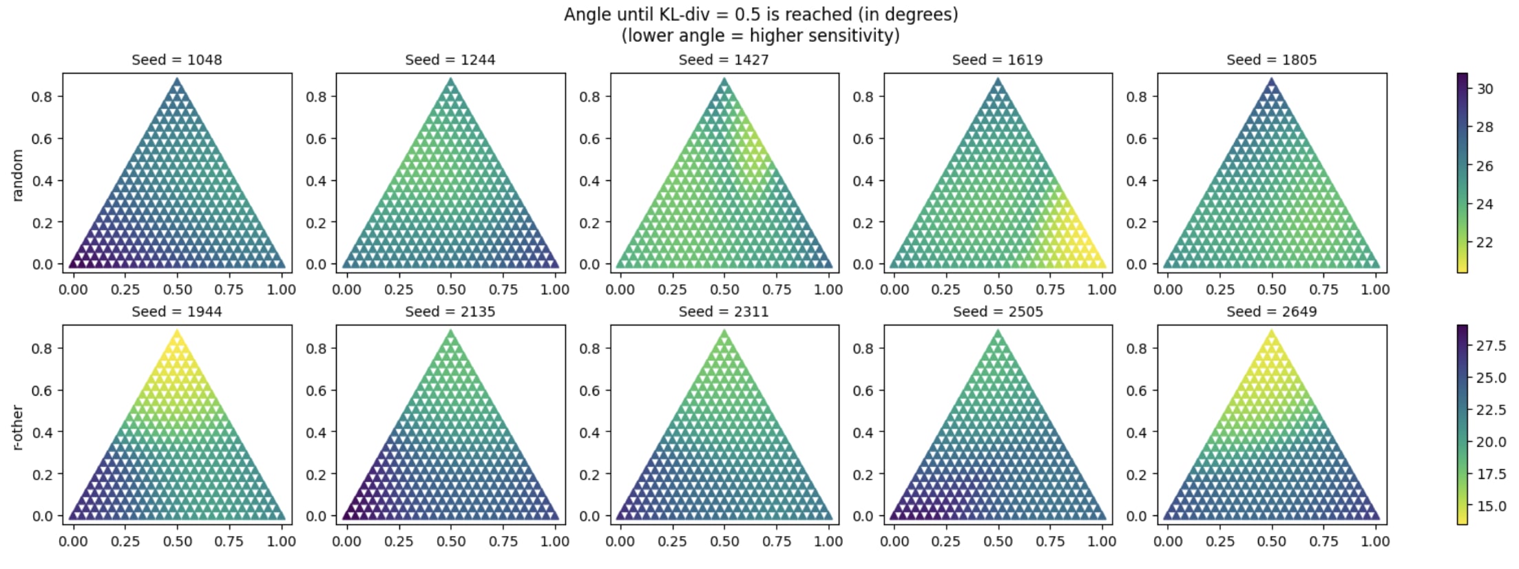
While these plots initially seem to suggest a local optimum at the top corner (2nd row), they only test two (random) directions in 768d space. If real-other directions consist of ~L0 number of features, and the previous hypothesis is true, we expect there to be an L0-dimensional space in which the direction is not a local optimum. We plan to continue these investigations in future work.

1. ^{^}

   Empirically this is a bit messy: Inputting a random direction into an SAE activates between 10 and 20000 features (lognormal distribution with a peak around 30). But that is using the encoder, I'm not sure if I should be doing that.

2. ^{^}

   The real-other direction is expected to turn on some features, but also to dampen existing features. My explanation focuses on turning on inactive features, and ignores the slight dampening of active features.

3. ^{^}

   This is not fully true—we know some directions represent non-sparse positional features, and there is information in the geometry of features—but we leave this aside for now.

Discuss