本文深入探讨了神经网络的记忆和泛化能力，通过引入“电路桶”的概念，将神经网络视为一组电路的集合。每个电路都有其复杂度和准确率，二者之间的比率定义了学习系数，而其倒数则表示电路的效率。文章还介绍了局部效率谱和学习系数谱，并提出了通过“退火”过程来逆向理解学习过程。文章通过几个玩具模型，如纯记忆、模加法和线性回归等，展示了不同电路的效率和学习行为，为理解神经网络的学习机制提供了新的视角。

💡神经网络可以被视为一组电路的集合，每个电路都有其特定的复杂度和准确率。

📈电路的效率定义为准确率与复杂度的比率，效率高的电路在学习过程中更倾向于被保留。

🌡️“退火”过程，通过引入噪声逐步关闭效率较低的电路，可以逆向理解神经网络的学习过程，揭示了学习过程中电路的激活顺序。

🧮在模加法和线性回归等模型中，存在记忆电路和泛化电路，记忆电路效率较低但复杂度也低，泛化电路则相反，这解释了神经网络学习过程中的不同阶段。

🧩文章提出了一个“电路桶”的视角，为理解神经网络的记忆和泛化能力提供了新的框架，并为未来的实验设计提供了理论基础。

Published on January 29, 2025 3:06 PM GMT

This is “Part I.75” of my series on the memorization-generalization spectrum and SLT.

I’m behind on some posts, so I thought I would try to explain, in a straightforward and nontechnical way, the main takeaway from my previous post for people thinking about and running experiments with neural nets. I’m going to punt on some technical discussions (in particular the discussion on SLT-type phenomenon related to “degrading a single circuit” and a deeper discussion of “locality”), and give an informal explanation of local efficiency spectra and the associated spectrum of (local) learning coefficients. 

I will next list a few predictions – both “purely cartoon” predictions, and how they are complicated by reality – about experiments. In one case (that of modular addition), the experiment is something I have done experiments on with Nina Panickssery (and confirms the prediction here); in another case (linear regression), there are several experiments confirming the SLT prediction. In the other cases, the learning coefficient spectrum has not been measured as far as I know. I would be very interested in experiments tackling this, and would be happy to either collaborate with anyone who’s interested in working out one of these or let anyone interested run the experiment (and perhaps reference this post). Note that this is far from a “carefully optimized” set of toy examples: I would also be excited for people to come up with their own.

Two-dimensional circuit efficiency spectra: redux

A takeaway from the previous two parts is that, in a certain reductionist operationalization, one can model a neural nets as “aggregating a bucket of circuits”. Each circuit has two key parameters. 

Its complexity. This is more or less the description length (e.g. in binary). More precisely, it is the “number of bits” that need to be tuned correctly to specify the circuit^[1].Its accuracy. The relevant measurement of accuracy is a bit tricky and the “units” need to be right. It can be approximated to the very rough level we care about here as the “log odds ratio” of a classification task being correct, or the (negative) “log loss” in an MSE (mean-squared-error) approximation task.

We plot the “bucket of circuits” on a 2-dimensional graph. Here a “cross” at (x,y) corresponds to a circuit with complexity x and log error parameter y. 

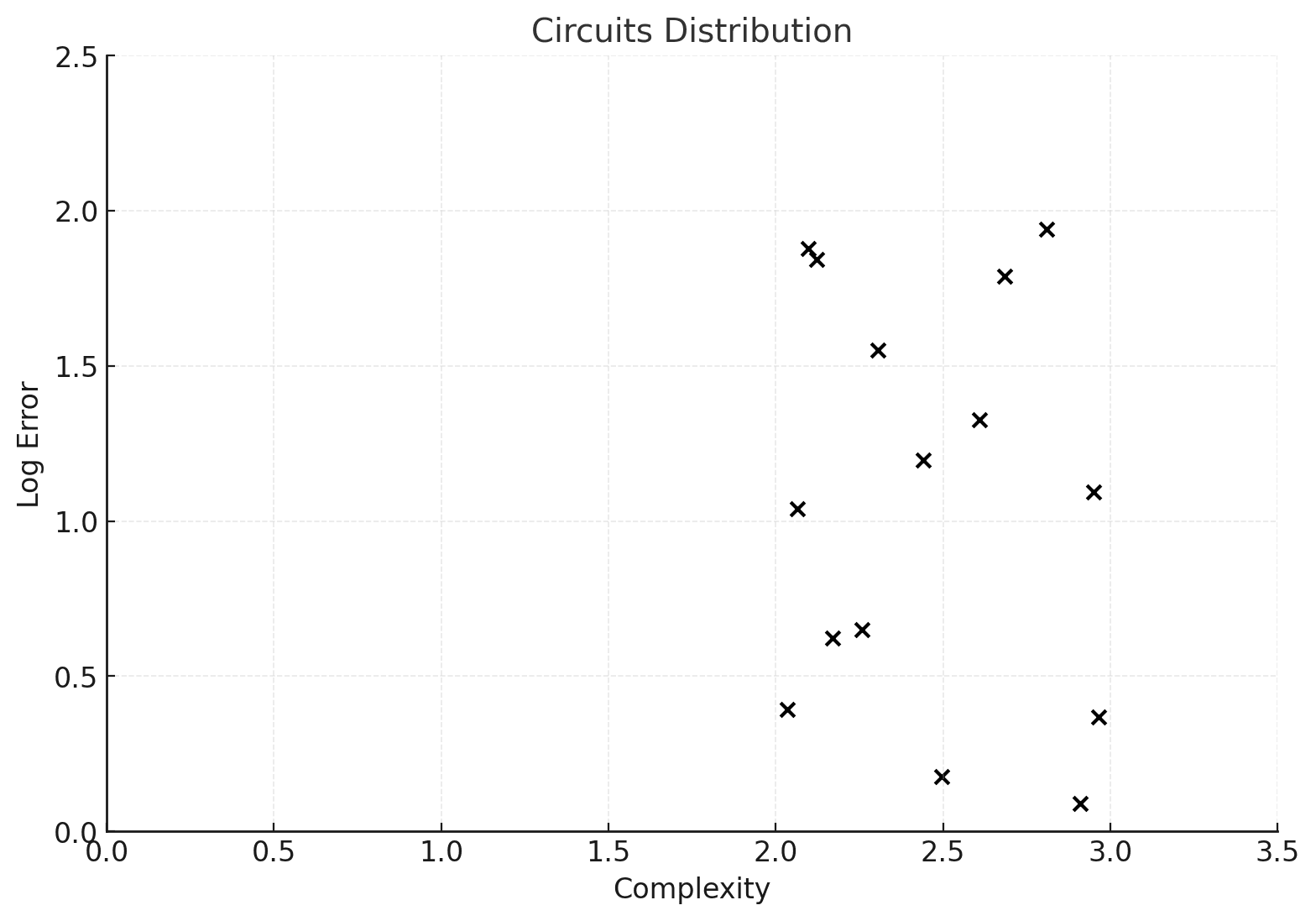
This is a cartoon and I’m not being careful at all about units (so assume that the x and y coordinates are suitably rescaled from a more realistic example). In fact in most contexts it is possible to view the two measurements in the same units and the complexity will tend to be significantly higher than the log error. The quotient, complexity/error of a circuit, is called the learning coefficient:

$$\lambda \left(C\right)=\frac{\text{Complexity}\left(C\right)}{\text{Log Error}\left(C\right)}.$$

It is a measure of “effective dimension”, as is well-known in SLT and as I’ll explain in the next installment. For this applied post, I won’t care about that. In fact, here it will be more intuitively useful to think of the inverse measurement, which measures the efficiency of a circuit:

$$\text{Eff}\left(C\right)=\frac{1}{\lambda \left(C\right)}=\frac{\text{Log Error}\left(C\right)}{\text{Complexity}\left(C\right)}.$$

The efficiency is the slope of the line connecting a circuit C to the origin in the graph above.

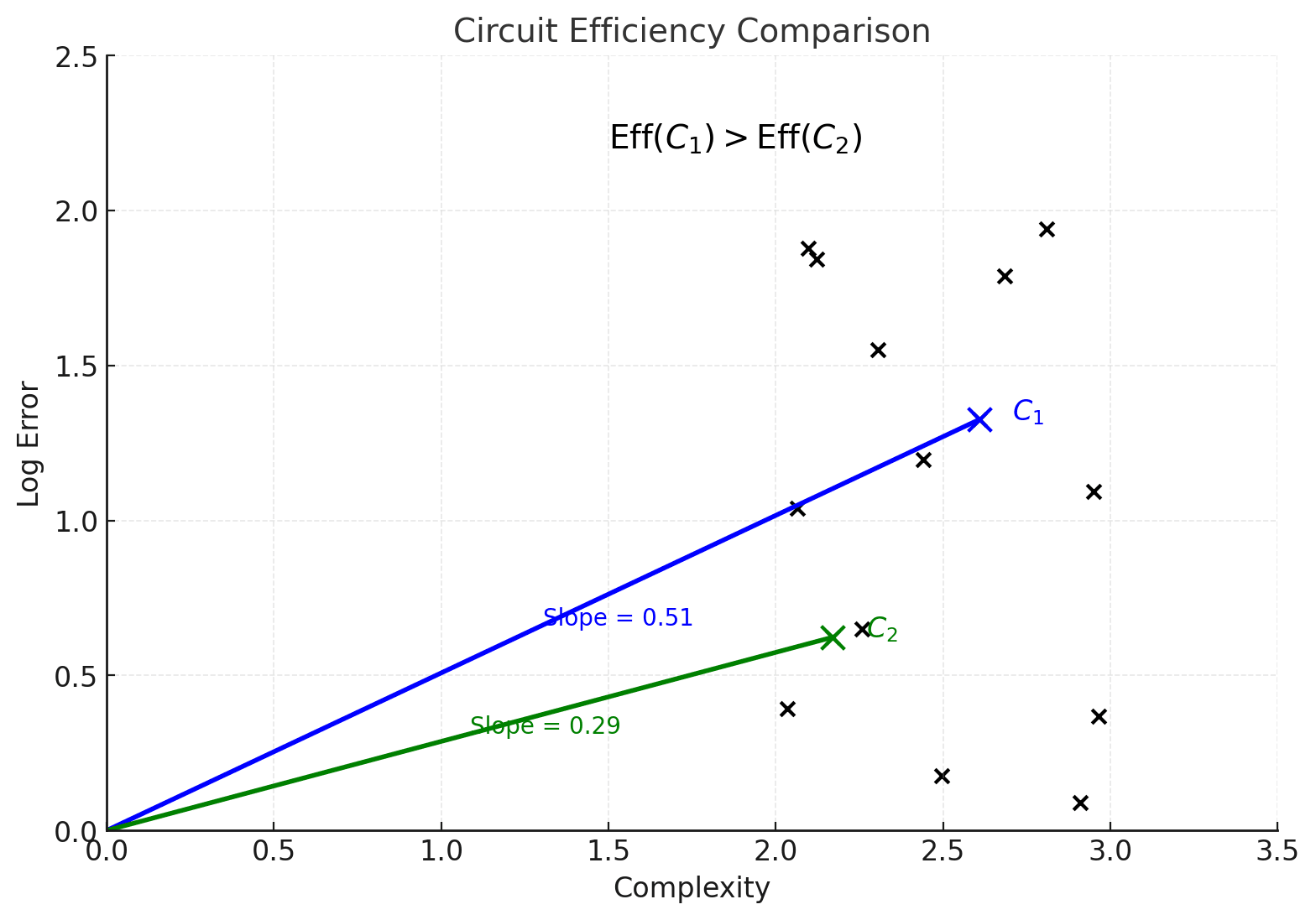
Here we’ve isolated a pair of circuits and drawn their slopes. Even though the blue circuit $C_1$ is more complex than the green circuit $C_2$, it is more efficient as it has larger slope – it corresponds to a more favorable tradeoff of accuracy to error reduction.

Now as I explained last time, one can trace through circuits in reverse order of efficiency by turning on a “temperature” parameter to trace through the rate-distortion curve. I won’t discuss here what temperature means or what the rate-distortion curve represents. But the takeaway is that via numerical sampling algorithms like “SGLD”, used by SLT practitioners, we can implement process called (local) tempering, which (in a cartoon approximation), gradually and carefully introduces noise to turn off circuits one by one, starting from the most inefficient ones, and ending up with only noise. Below I show a snapshot of the “surviving circuits” (in red) in the middle of the tempering process.

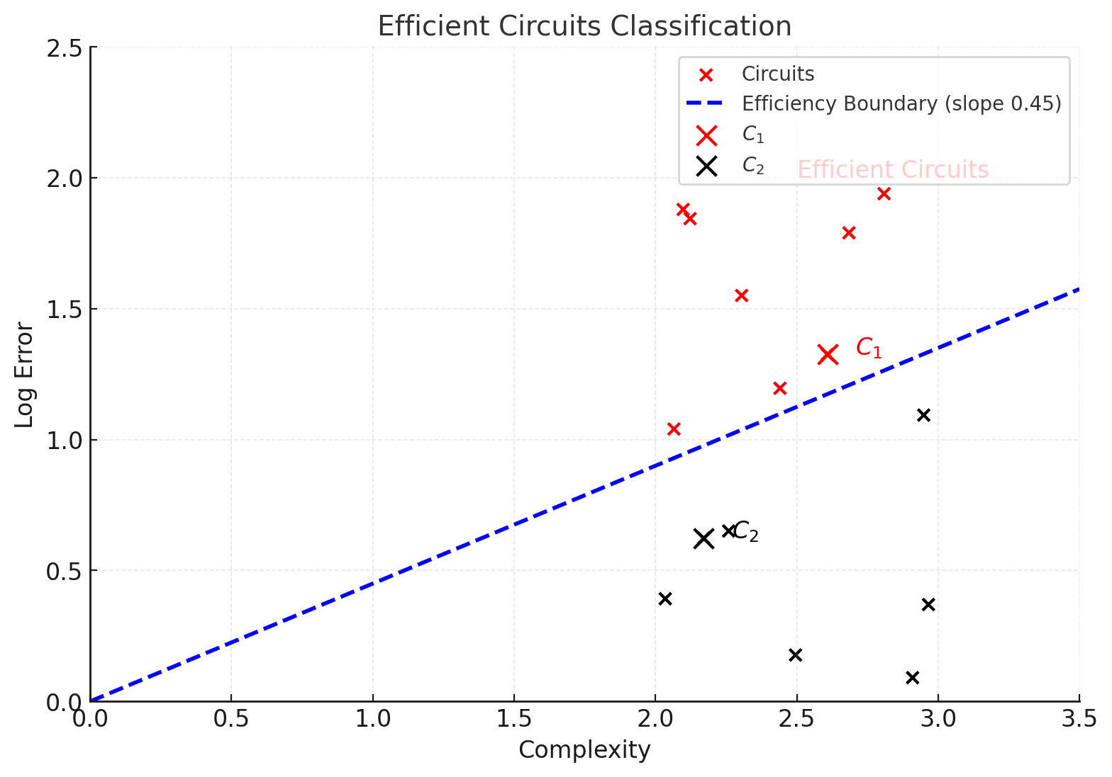
Here $C_1$ has survived tempering and $C_2$ has been noised out. As tempering proceeds, the blue “efficiency line” sweeps counterclockwise, noising out more and more circuits (black) and retaining fewer and fewer survivors (red).

I also explained last time that tempering can be thought of as an ersatz cousin of learning but with opposite sign. Very roughly, tempering is a kind of “learning process in reverse”, starting with a “fully learned” algorithm and forgetting components as tempering proceeds. However it’s important to note that the two are subtly different, with “tempering” associated to thermostatic phenomena (cognate: “Bayesian learning”) and “learning” associated to thermodynamic ones (cognate: “SGD”). 

In particular, while tempering only cares about efficiency, learning cares much more about complexity. In a very rough (and not-entirely-accurate) cartoon, we can think of going forwards in learning (e.g. think of this as checkpoints in a learning trace) as tuning the complexity parameter only. Below we see an example of a cartoon learning snapshot. This time circuit $C_2$ is learned (red) and circuit $C_1$ is not yet learned (black), despite $C_1$ being more efficient.

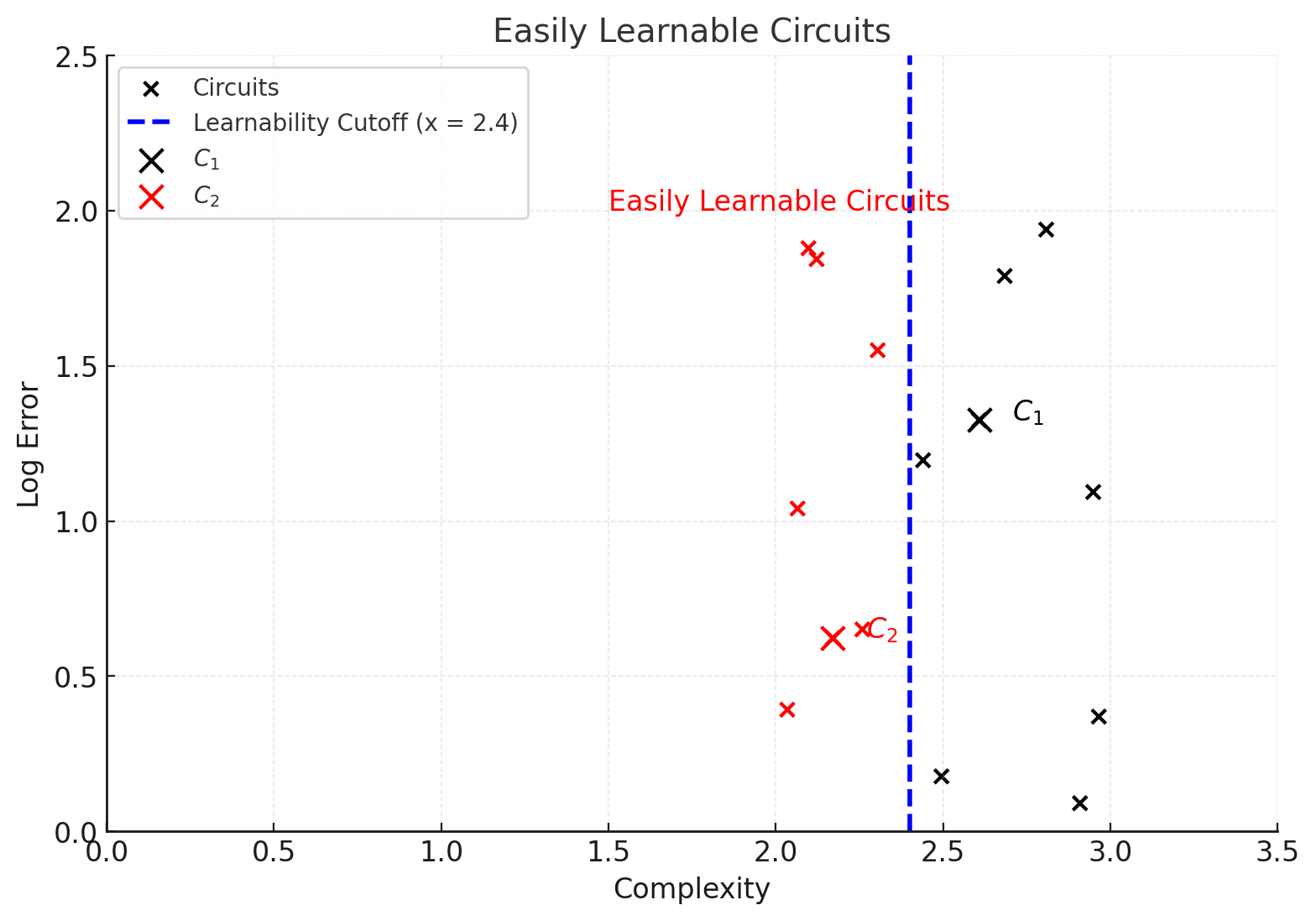
We’re abstracting away lots of stuff: in “reality” there are issues of interdependence of sequential circuits (and in fact problematicity of the very notion of a “circuit”), we are modeling as a discrete “off vs. on” process something that is in fact a more gradual / continuous thing, etc. But modulo all this, we’ve made a “cartoon picture” of learning and tempering. Note that this cartoon picture makes approximate predictions. It predicts that in each of these settings, only the “red” circuits contribute to empirical measurements of complexity and error. So the total loss is (very approximately, and ignoring some small factors) equal to the exponent of the total log error of the red circuits, and the total complexity (empirically extractable as a free energy measurement) is the sum of the complexities of the red circuits. 

Cartoons for toy models

Now I’m going to draw the “cartoons” as above for a few toy models. Some are known, and some are my predictions. Everything is to be understood very roughly and asymptotically: I’m happily ignoring factors of O(1) and even sometimes “logarithmic factors”.

Pure memorization

In the picture above, our bucket of circuits was spread out among the x-y plane. In reality, a lof of the time we’ll see models with big clusters of circuits with roughly the same error and complexity. This is most obvious in a “pure memorization” picture, where we assume there is some finite set of $D$ possible datapoints to learn, with no way to compress the outputs of the computation. Here each memorization circuit approximately multiplies the odds by $1-1/D,$ so its log-error is $\frac{1}{D}$^[2].

In a naive model of a boolean classifier, each memorization costs “1 bit of complexity”. Thus we get the following “bucket of circuits” spectrum for a pure-memorization process:

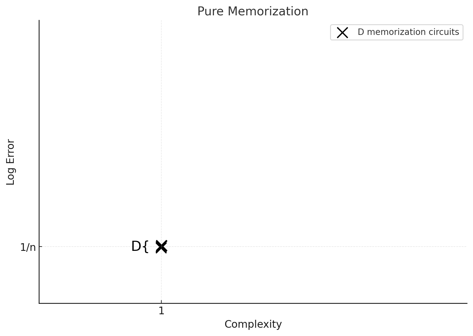
The “fat cross” houses D different circuits, all with the x- and y- values, associated to memorizing one of the D different datapoints.

Modular addition and linear regression

The modular addition model learns to add two residues modulo a prime p. I’m going to assume that we’ve trained modular addition on the full dataset of $$D=p^2.$$ A modular addition model can memorize up to $D=p^2$ values, and each leads to a $\frac{1}{p^2}$ improvement in the log-odds. It can implement a number of “generalizing” circuits, which have complexity $O\left(p\right)$ but lead to nontrivial improvement for all inputs, thus an $O\left(1\right)$ improvement. 

 

Here I’m drawing a cartoon of a model that has memorized some number m of inputs and also learned some quantity, k, of “generalizing circuits”. In the cartoon below I used the (unrealistically small) value p = 3 to generate the picture, but it represents a much larger “asymptotic” picture.

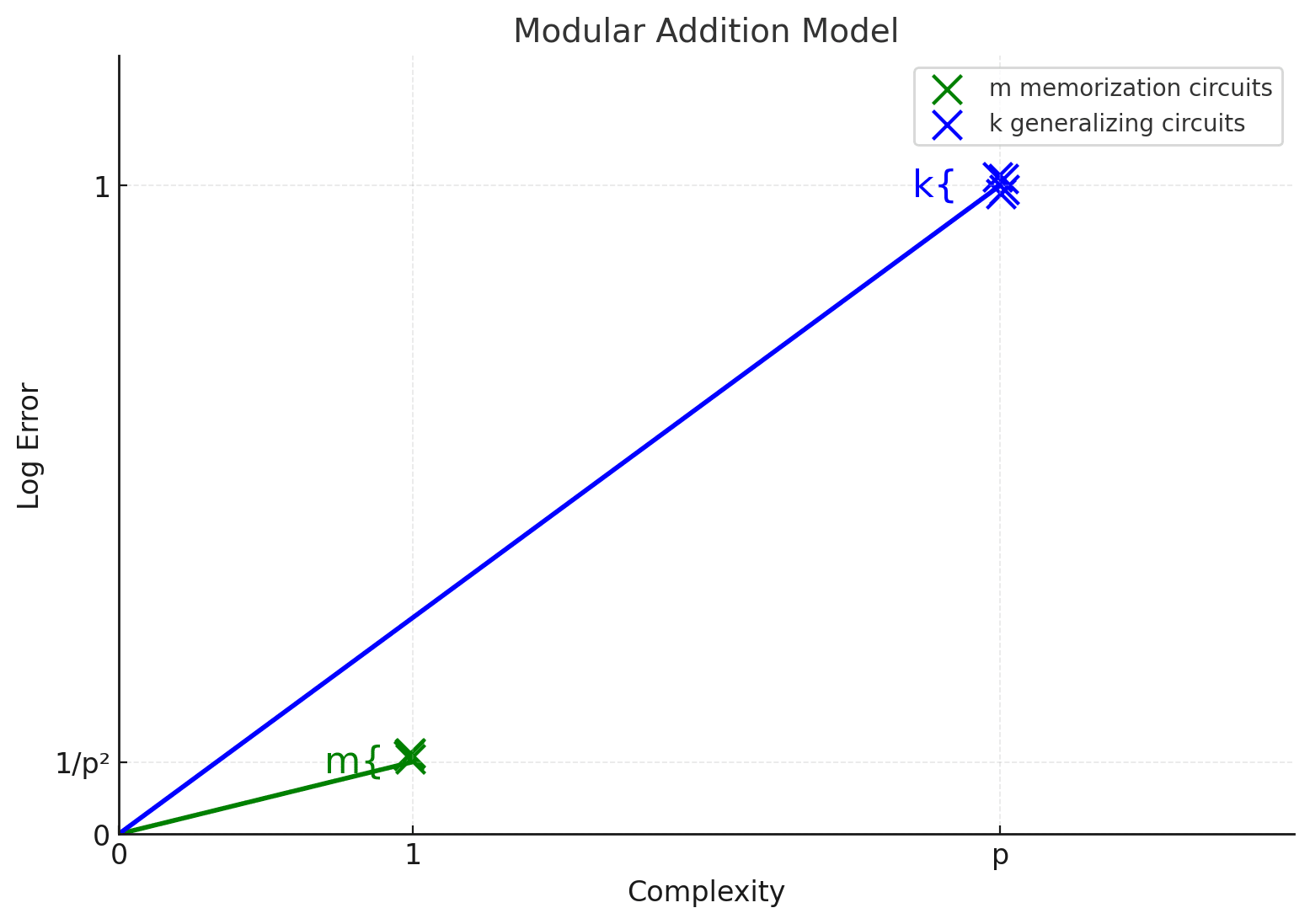
Here we observe that memorizing circuits are less efficient, but have lower complexity – thus they are both the first to be learned and the first to be forgotten when we turn on tempering on the fully-learned model. In our work on the subject with Nina we observed exactly this behavior, with a surprisingly exact fit of the learning coefficient to the (inverse) slopes predicted by this naive “bucket of circuits” picture.

A similar picture, with a bunch of memorizing circuits and a single generalizing circuit, takes place for linear regression. We’ll see in the next installment that both the linear regression and the memorization picture have an additional phenomenon, where “memorization circuits” can be learned to varying levels of numerical precision: thus each circuit actually has some “spread” where by tuning parameters to be more vs. less precise, it can further trade off complexity vs. error. In both instances, to first order this effect actually has the same efficiency (i.e. the same slope and “learning coefficient”) as the more naive “discrete” picture. 

Prefix matching

Now let’s look at the “prefix matching” model introduced in the second half of my first post in this series. Feel free to skip this if you haven’t read that post. Here we saw that the circuits actually split up into 10 different “memorization-shaped” phenomena associated to memorizing prefixes of various length. Since the picture there had exponential scale, it would be hard to fit all of them visibly on the same diagram, and I’ll only draw the first 4 “buckets” of prefix-matching behaviors. I’ll just draw the expected cartoon here; unlike in the very naive analysis in that post, I’m going to include in this cartoon the observation that memorizing a prefix in an n-letter alphabet of length k requires about k log(n) bits. So the “complexity” scale will be in factors of log(n). (I’m slightly inconsistently log-order complexity differences in this very cartoon picture):

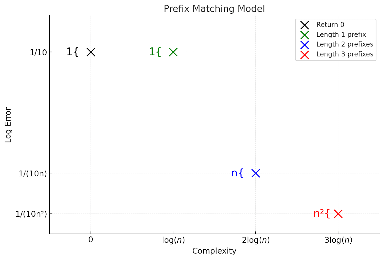
I again set n = 3 for plotting purposes. Here we see:

There is now a spectrum of behaviors from “more generalization-like” circuits with higher efficiency to “more memorization-like” circuits with low efficiency.Another difference from the examples in the last section is that memorization behaviors have higher complexity here. So circuits we expect to get learned sooner actually also should survive longer into tempering (have higher “efficiencies”, i.e., slopes).We can extract a predicted rough spectrum of learning coefficients here; up to log and constant factors, we for instance expect a circuit implementing all of these behaviors (but not circuits associated to higher prefix lengths) to roughly have slope $\sim \frac{1}{n^2}$, corresponding to a learning coefficient of $$\lambda \sim \frac{1}{1/n^2}=n^2.$$

 

Fourier monomials

While this is a slightly different context, I expect a similar (but much less extreme) behavior to prefix matching to occur in learning low-degree polynomials in the boolean Fourier basis in a setup like the “leap complexity” paper.  Here the prediction task is to approximate a Fourier polynomial: something like $$F\left(b\right)=1+b_1+b_2\cdot b_3$$ on a length-n $\pm 1$-valued boolean word $b=(b_1,b_2,\dots ,b_n)$, with $b_i\in \pm 1$ (note that the coefficients here are signed rather than 0 or 1; they’re sometimes written as $(-1{)}^b$ for usual booleans $b\in \{0,1\}$) . Circuits are associated to learning a single monomial (there are two monomials in the above picture). Specifying a monomial of degree d requires specifying d coordinates between 0 and n. So roughly, we expect a similar behavior:

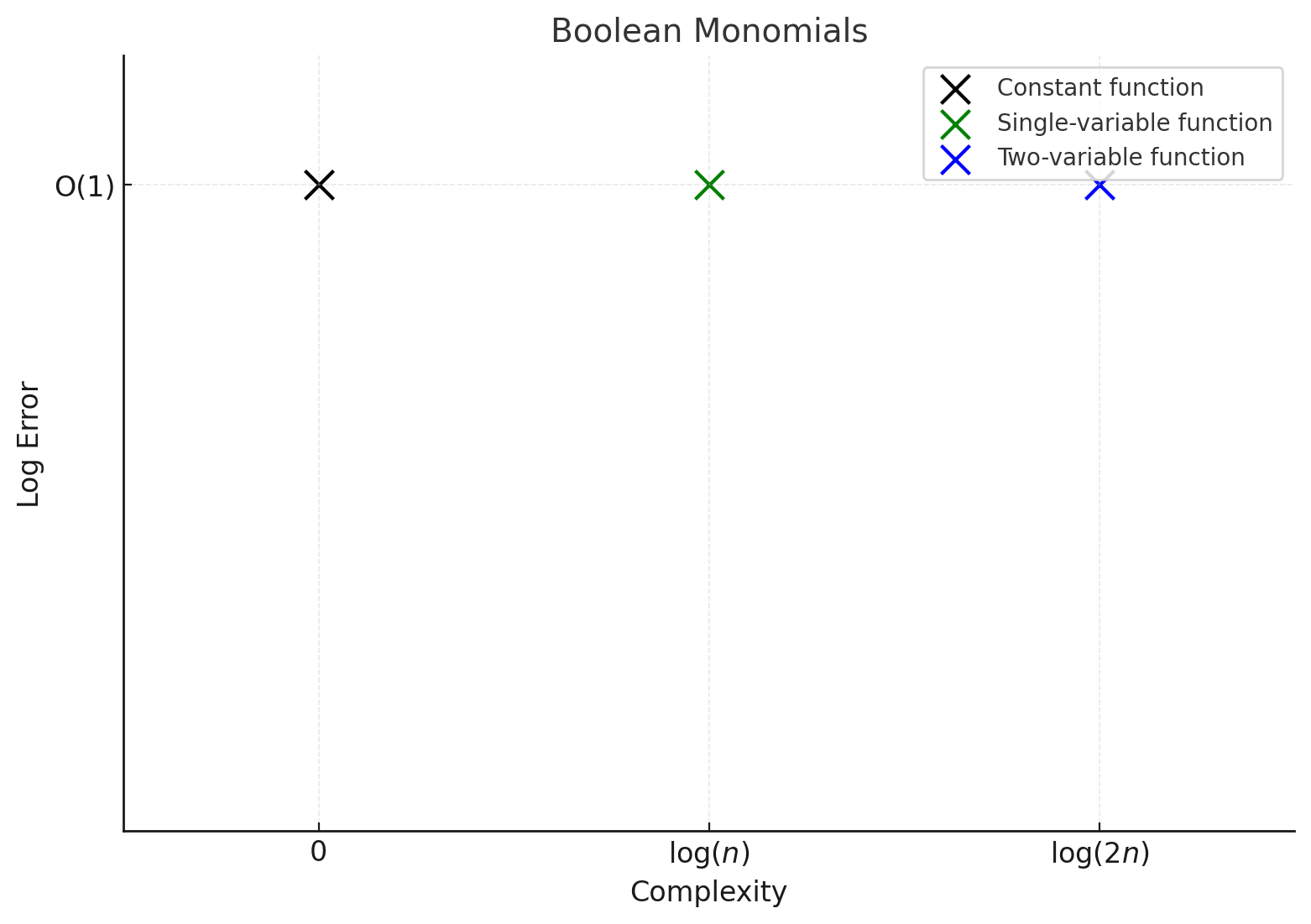
Here again, efficiency correlates with learnability. But an interesting prediction of that paper is that in fact, the learnability of a higher-degree monomial depends significantly on whether it is a multiple of a previously learned monomial. So the polynomial $1+b_1+b_2\cdot b_3$ above takes asymptotically much longer to learn than $1+b_1+b_1\cdot b_2$, though they have the same circuit efficiency diagrams (and then “parity learning” issues imply that even a single monomial of sufficiently high degree is simply impossible to learn in polynomial time). Thus while I claim these diagrams give lead to pretty strong “thermostatic” predictions about tempering and learning coefficient spectra, the “thermodynamic” questions of learning are generally much trickier and even in the simplest toy cases with reasonably well-behaved circuit decompositions, they cannot be simply read off (even approximately) from the complexity and accuracy values in these “bucket of circuits” cartoon pictures. 

1. ^{^}

   We specifically think in terms of the formal “Solomonoff complexity” or “entropy” measure; this is not exactly the same as the “number of bits” or “OOM precision of linear parameters”, and this is interesting – e.g. SLT has a lot of stuff to say here. But in all examples here, and to the “cartoon” accuracy we use, very simple notions of complexity will be sufficient.

2. ^{^}

   Since memorizations combine additively, a multiplicative error picture doesn’t quite apply here; however, if we’re only looking at the first few memorizations, and we’re happy to ignore subleading corrections, this is a reasonable model.

Discuss