文章探讨了Markov's不等式，介绍其公式及特点，阐述了它作为尾界的优势与局限性，还提到它与Chebyshev's不等式、Chernoff bound的关系，以及证明过程中的要点。

🎯Markov's不等式：P(X≥a)≤E[X]/a，适用于非负随机变量

💪作为尾界，可在不知方差时控制随机变量尾行为，但界限不紧

🤝与Chebyshev's不等式、Chernoff bound有关，体现其重要性

🧐证明过程中需注意将概率分布分为两区域，及非负性的作用

Published on January 8, 2025 12:31 AM GMT

In my experience, the proofs that you see in probability theory are much shorter than the longer, more involved proofs that you might see in other areas of math (like e.g. analytical number theory). But that doesn't mean that good technique isn't important. In probability theory, there are a set of tools that are useful across a broad variety of situations and you need to be able to recognize when it's the appropriate time to use each tool in your toolkit.

One of the most useful of tools to have is Markov's inequality. What Markov's inequality says is that, given a non-negative random variable $X$and a positive real number $a$, the probability that $X$ is greater than $a$ can be upperbounded in the following manner:

$$P(X\ge a)\le \frac{E\left[X\right]}{a}$$

This is a pretty simple formula. You might have even been able to guess it beforehand using dimension analysis. Probabilities are often thought of as dimensionless quantities. The expectation $E\left[X\right]$ and the threshold $a$ both have units of "length", so we would need them to exactly cancel out to create a dimensionless quantity. We naturally expect that the probability of exceeding the threshold to (a) increase as the expectation of $X$ increases and (b) decrease as the value of the threshold $a$ increases. These sorts of arguments alone would point you in the direction of a formula of the form:

$$P(X\ge a)\le {\left(\frac{E\left(X\right)}{a}\right)}^k$$

Why does $k$ equal $1$ in the case of Markov's inequality? There is probably some elegant scaling argument that uniquely pins down the power $k$, but we won't dwell on that detail.

Markov's inequality might not seem that powerful, but it is. For two reasons:

One reason is that Markov's inequality is a "tail bound" (a statement about the behavior of the random variable far away from its center) that makes no reference to the variance. This has both its strengths and its weaknesses. The strength is that there are many situations where we know the mean of a random variable but not its variance, so Markov's inequality is the only tool in our repertoire that will allow us to control the tail behavior of the variable. The weakness is that because it assumes nothing about the variance (or any higher moments), Markov's inequality is not a very tight bound. If you also know the variance of your random variable, you can do much better (though you will need more heavy-duty techniques like moment-generating functions).

The other reason why Markov's inequality is powerful is that, in a sense, many properties of random variables are just statements about the mean (the expectation) of some other random variable.

For example, the variance of a random variable $X$ is nothing more than the expectation of the random variable $Y=(X-\mu {)}^2$ where $\mu$ is the mean of $X$. Let's say we know that the variance of $X$ is ${\sigma }^2$. Because $Y$ is a non-negative random variable, it follows that $\sqrt{Y}=|X-\mu |$ is well-defined and also a non-negative random variable. We can then show that:

$$\begin{array}{cc}P(|X-\mu |\ge k\sigma )& =P(\sqrt{Y}\ge k\sigma )\\ & =P(Y\ge k^2{\sigma }^2)\\ & \le \frac{E\left(Y\right)}{k^2{\sigma }^2}\\ & =\frac{1}{k^2}\end{array}$$

This relationship is special enough that it has its own name: Chebyshev's inequality. But it's just Markov's inequality in disguise! Let's do one more.

We can define the parametrized set of random variables $Z\left(t\right)=e^{tX}$. The parametrized set of expectations $M\left(t\right)=E\left[Z\right(t\left)\right]$ has a name called the moment-generating function (because if you take derivatives of $M\left(t\right)$ with respect to $t$ and evaluate at $t=0$, you get the moments of the original random variable $X$). We then have that:

$$\begin{array}{cc}P(X\ge a)& =P(e^{tX}\ge e^{ta})\\ & \le \frac{E\left[e^{tX}\right]}{e^{ta}}\\ & =M\left(t\right)e^{-ta}\end{array}$$

Hey, that's the Chernoff bound!

Despite being fairly simple as math goes, it took a couple of exposures for Markov's inequality to properly stick with me. To see why, let's walk through the proof which conceptually involves two steps.

Let's say we have a threshold $a$. We want to divide the probability distribution of $X$ into two regions: $x<a$ and $x\ge a$.

If we take all of the probability mass for values of $x$ larger than $a$ and smush it at $a$, then the new distribution will have an expectation which is less than or equal to the expectation of $X$.

Similarly, if we take the probability mass for all points $x<a$ and smush it to $x=0$, then the new distribution will also have an expectation less than or equal to the previous one.

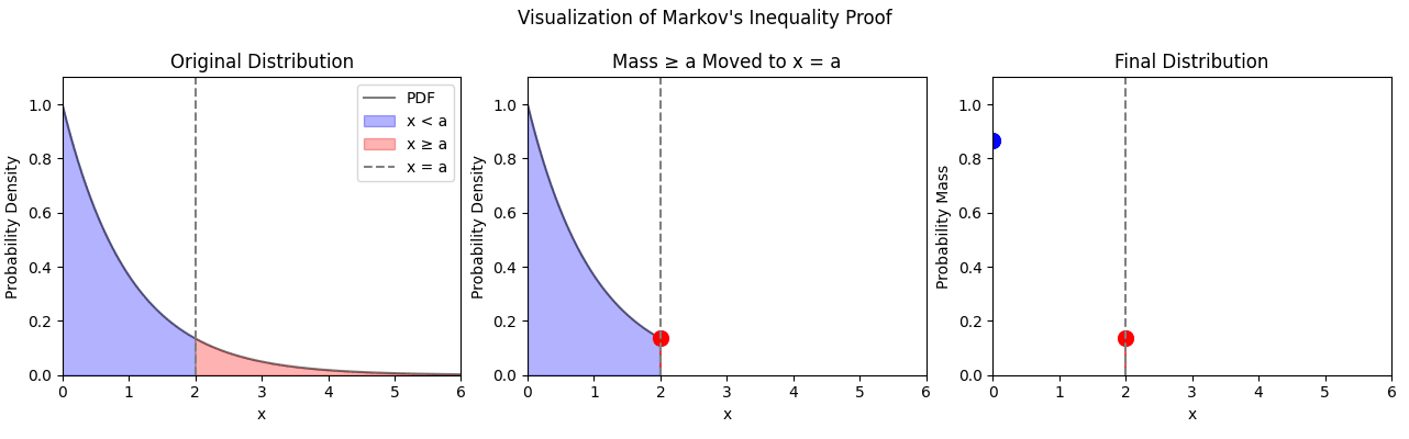
What is the expectation of this final distribution? There would be two contributions to the expectation: the probability mass at $x=0$ multiplied by 0 and the probability mass at $x=a$ multiplied by $a$. The first term vanishes so we are left with an overall expectation $P(X\ge a)\cdot a$. We can then compare this expectation to the expectation of our original distribution and then divide by $a$ to get Markov's inequality:

$$P(X\ge a)\cdot a\le E\left[X\right]⟶P(X\ge a)\le \frac{E\left[X\right]}{a}$$

Well this is a simple proof. Where did I struggle before?

An important thing to keep in mind is that Markov's inequality only holds for non-negative random variables. The first part of the proof is easy for me to remember because $a$ sticks out to me as an obvious threshold to smush probability mass to. But the second part where we smush all the mass to $0$ used to elude me because I didn't keep in mind that the non-negativity of $X$ makes $0$ a kind of threshold as well.

Discuss