
Gated Multimodal Units for Information Fusion
Deep learning has proven its superiority in many domains, in a variety of tasks such as image classification and text generation. Dealing with tasks that involve inputs from multiple modalities is an interesting research area.
The Gated Multimodal Unit (GMU) is a new building block proposed by a recent paper, which is presented in ICLR 2017 as a workshop. The goal of this building block is to fuse information from multiple different modalities in a smart way.
In this post I'll describe the GMU, and illustrate how it works on a toy data set.
The architecture
Given two representations of different modalities, $x_v$ and $x_t$ (visual and textual modalities for instance), the GMU block performs a form of self attention: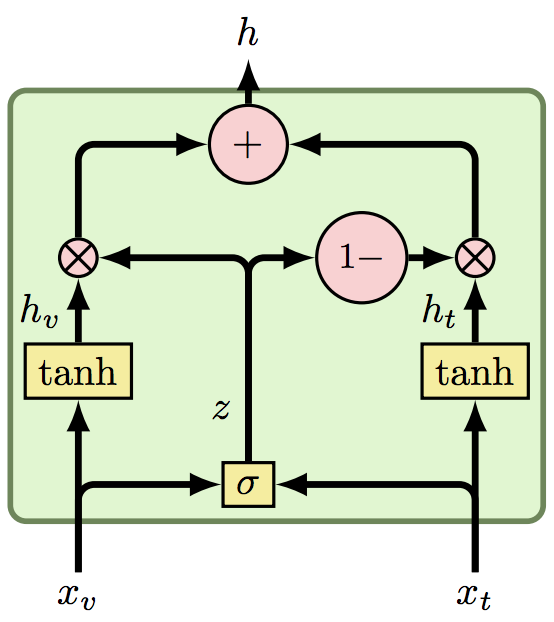
The equations describing the GMU are relatively simple:
(1) $h_v = tanh(W_v \cdot x_v)$
(2) $h_t = tanh(W_t \cdot x_t)$
(3) $z = \sigma(W_z \cdot [x_v, x_t])$
(4) $h = z \cdot h_v + (1 - z) \cdot h_t$
(1) + (2) are transforming the representations into different representations, which are then attended in (4) according to $z$ which is calculated in (3). Since $z$ is a function of $x_v$ and $x_t$, it means we're dealing with a self attention mechanism.
The intuition behind the GMU is that it uses the representations themselves to understand which of the modalities should affect the prediction. Consider the task of predicting the gender of a photographed person accompanied by a recording of his voice. If the recording of a given example is too noisy, the model should learn to use only the image in that example.
Synthetic data
In the paper they describe a nice synthetic data set which demonstrates how the GMU works.
Here we'll implement the same data set, and find out for ourselves whether or not the GMU actually works (spoiler alert: it does).
First, let's do the imports:
import tensorflow as tfimport numpy as npimport matplotlib.pyplot as pltnp.random.seed(41)tf.set_random_seed(41)%matplotlib inlineGenerate the data

Don't let the graph scare you - later on you'll find a visualization of the data generated by this graph.
Basically what the graph says is that the target class $C$ depicts the values of the modalities $y_v$ and $y_t$ - with some randomness of course.
In the next step the random variable $M$ decides which of the inputs $y_v$, $y_t$ to ignore, and instead to use a source of noise $\hat{y}_v$, $\hat{y}_t$.
In the end, $x_v$ and $x_t$ contain either the real source of information which can describe the target class $C$, or random noise.
The goal of the GMU block is to successfully find out which one of the sources is the informative one given a specific example, and to give all the attention to that source.
n = 400p_c = 0.5p_m = 0.5mu_v_0 = 1.0mu_v_1 = 8.0mu_v_noise = 17.0mu_t_0 = 13.0mu_t_1 = 19.0mu_t_noise = 10.0c = np.random.binomial(n=1, p=p_c, size=n)m = np.random.binomial(n=1, p=p_m, size=n)y_v = np.random.randn(n) + np.where(c == 0, mu_v_0, mu_v_1)y_t = np.random.randn(n) + np.where(c == 0, mu_t_0, mu_t_1)y_v_noise = np.random.randn(n) + mu_v_noisey_t_noise = np.random.randn(n) + mu_t_noisex_v = m * y_v + (1 - m) * y_v_noisex_t = m * y_t_noise + (1 - m) * y_t# if we don't normalize the inputs the model will have hard time trainingx_v = x_v - x_v.mean()x_t = x_t - x_t.mean()plt.scatter(x_v, x_t, c=np.where(c == 0, 'blue', 'red'))plt.xlabel('visual modality')plt.ylabel('textual modality');Create the model
I'll implement a basic version of the GMU - just to make it easier to comprehend.
Generalizing the code to handle more than two modalities is straightforward.
NUM_CLASSES = 2HIDDEN_STATE_DIM = 1 # using 1 as dimensionality makes it easy to plot z, as we'll do later onvisual = tf.placeholder(tf.float32, shape=[None])textual = tf.placeholder(tf.float32, shape=[None])target = tf.placeholder(tf.int32, shape=[None])h_v = tf.layers.dense(tf.reshape(visual, [-1, 1]), HIDDEN_STATE_DIM, activation=tf.nn.tanh)h_t = tf.layers.dense(tf.reshape(textual, [-1, 1]), HIDDEN_STATE_DIM, activation=tf.nn.tanh)z = tf.layers.dense(tf.stack([visual, textual], axis=1), HIDDEN_STATE_DIM, activation=tf.nn.sigmoid)h = z * h_v + (1 - z) * h_tlogits = tf.layers.dense(h, NUM_CLASSES)prob = tf.nn.sigmoid(logits)loss = tf.losses.sigmoid_cross_entropy(multi_class_labels=tf.one_hot(target, depth=2), logits=logits)optimizer = tf.train.AdamOptimizer(learning_rate=0.1)train_op = optimizer.minimize(loss)Train the model
sess = tf.Session()def train(train_op, loss): sess.run(tf.global_variables_initializer()) losses = [] for epoch in xrange(100): _, l = sess.run([train_op, loss], {visual: x_v, textual: x_t, target: c}) losses.append(l) plt.plot(losses, label='loss') plt.title('loss') train(train_op, loss)Inspect results
The loss is looking good.
Let's look what $z$ and the predictions look like. The following visualizations appear in the paper as well.
# create a mesh of points which will be used for inferenceresolution = 1000vs = np.linspace(x_v.min(), x_v.max(), resolution)ts = np.linspace(x_t.min(), x_t.max(), resolution)vs, ts = np.meshgrid(vs, ts)vs = np.ravel(vs)ts = np.ravel(ts)zs, probs = sess.run([z, prob], {visual: vs, textual: ts})def plot_evaluations(evaluation, cmap, title, labels): plt.scatter(((x_v - x_v.min()) * resolution / (x_v - x_v.min()).max()), ((x_t - x_t.min()) * resolution / (x_t - x_t.min()).max()), c=np.where(c == 0, 'blue', 'red')) plt.title(title, fontsize=14) plt.xlabel('visual modality') plt.ylabel('textual modality') plt.imshow(evaluation.reshape([resolution, resolution]), origin='lower', cmap=cmap, alpha=0.5) cbar = plt.colorbar(ticks=[evaluation.min(), evaluation.max()]) cbar.ax.set_yticklabels(labels) cbar.ax.tick_params(labelsize=13) plt.figure(figsize=(20, 7))plt.subplot(121)plot_evaluations(zs, cmap='binary_r', title='which modality the model attends', labels=['$x_t$ is important', '$x_v$ is important'])plt.subplot(122)plot_evaluations(probs[:, 1], cmap='bwr', title='$C$ prediction', labels=['$C=0$', '$C=1$'])We can see $z$ behaves exactly as we want (left figure). What's nice about it is that the class of points that reside far from the boundary line are predicted using practically only one of the modalities. It means the model learned when to ignore the modality that contains pure unpredictive noise.
Why not to use simple FF (Feed Forward)?
If we ignore the data generating process and just look at the data points, clearly there are 4 distinct clusters.
These clusters aren't linearly separable. While the GMU gives capacity to the model in order to explain this non-linear behaviour, one could just throw another layer to the mixture instead, thus solving the problem with plain feed-forward (FF) network.
The universal approximation theorem states that a feed-forward network with a single hidden layer containing a finite number of neurons, can approximate continuous functions... (Wikipedia)
So indeed, for this contrived example a simple FF will do the job. However, the point in introducing new architectures (GMU in this case) is to introduce inductive bias that allows the training process to take advantage of prior knowledge we have about the problem.
Conclusion
For real world problems involving multiple modalities, the authors claim the GMU achieves superior performance. They show cased their approach using the task of identifying a movie genre based on its plot and its poster.
GMU is easy to implement, and it may be worthwhile to keep it in your tool belt in case you need to train a model to use multiple modalities as input. To this end, you can create a sub network for each modality. The sub networks need not be the same - you can for instance use a CNN for a visual modality and LSTM for a textual one. What matters is that each sub network outputs a dense representation of its modality. Then, feed these representations into a GMU block in order to fuse the information into one representation. The fused representation will be fed into another sub network whose output will be the final prediction.
