

Optical Character Recognition (OCR) has revolutionized the way we interact with textual data in real life, enabling machines to read and interpret text from images, scanned documents, and handwritten notes. From digitizing books and automating data entry to real-time text translation in augmented reality, OCR applications are incredibly diverse and impactful. Some of its application may include:
- Document Digitization: Converts physical documents into editable and searchable digital formats.Invoice Scanning: Extracts details like amounts, dates, and vendor names for automated processing.Data Entry Automation: Speeds up workflows by extracting text from forms and receipts.Real-Time Translation: Translates foreign text from images or video streams in augmented reality.License Plate Recognition: Identifies vehicles in traffic systems and parking management.Accessibility Tools: Converts text to speech for visually impaired individuals.Archiving and Preservation: Digitizes historical documents for storage and research.
In this post, we take OCR a step further by building a custom OCR model for recognizing text in the Wingdings font—a symbolic font with unique characters often used in creative and technical contexts. While traditional OCR models are trained for standard text, this custom model bridges the gap for niche applications, unlocking possibilities for translating symbolic text into readable English, whether for accessibility, design, or archival purposes. Through this, we demonstrate the power of OCR to adapt and cater to specialized use cases in the modern world.
For developers and managers looking to streamline document workflows such as OCR extraction and beyond, tools like the Nanonets PDF AI offer valuable integration options. Coupled with state of the art LLM capabilities, these can significantly enhance your workflows, ensuring efficient data handling. Additionally, tools like Nanonets’ PDF Summarizer can further automate processes by summarizing lengthy documents.
Is There a Need for Custom OCR in the Age of Vision-Language Models?
Vision-language models, such as Flamingo, Qwen2-VL, have revolutionized how machines understand images and text by bridging the gap between the two modalities. They can process and reason about images and associated text in a more generalized manner.
Despite their impressive capabilities, there remains a need for custom OCR systems in specific scenarios, primarily due to:
- Accuracy for Specific Languages or Scripts: Many vision-language models focus on widely-used languages. Custom OCR can address low-resource or regional languages, including Indic scripts, calligraphy, or underrepresented dialects.Lightweight and Resource-Constrained Environments: Custom OCR models can be optimized for edge devices with limited computational power, such as embedded systems or mobile applications. Vision-language models, in contrast, are often too resource-intensive for such use cases. For real-time or high-volume applications, such as invoice processing or automated document analysis, custom OCR solutions can be tailored for speed and accuracy.Data Privacy and Security: Certain industries, such as healthcare or finance, require OCR solutions that operate offline or within private infrastructures to meet strict data privacy regulations. Custom OCR ensures compliance, whereas cloud-based vision-language models might introduce security concerns.Cost-Effectiveness: Deploying and fine-tuning massive vision-language models can be cost-prohibitive for small-scale businesses or specific projects. Custom OCR can be a more affordable and focused alternative.
Build a Custom OCR Model for Wingdings
To explore the potential of custom OCR systems, we will build an OCR engine specifically for the Wingdings font.
Below are the steps and components we will follow:
- Generate a custom dataset of Wingdings font images paired with their corresponding labels in English words.Create a custom OCR model capable of recognizing symbols in the Wingdings font. We will use the Vision Transformer for Scene Text Recognition (ViTSTR), a state-of-the-art architecture designed for image-captioning tasks. Unlike traditional CNN-based models, ViTSTR leverages the transformer architecture, which excels at capturing long-range dependencies in images, making it ideal for recognizing complex text structures, including the intricate patterns of Wingdings fonts.Train the model on the custom dataset of Wingdings symbols.Test the model on unseen data to evaluate its accuracy.
For this project, we will utilize Google Colab for training, leveraging its 16 GB T4 GPU for faster computation.
Creating a Wingdings Dataset
What is Wingdings?
Wingdings is a symbolic font developed by Microsoft that consists of a collection of icons, shapes, and pictograms instead of traditional alphanumeric characters. Introduced in 1990, Wingdings maps keyboard inputs to graphical symbols, such as arrows, smiley faces, checkmarks, and other decorative icons. It is often used for design purposes, visual communication, or as a playful font in digital content.
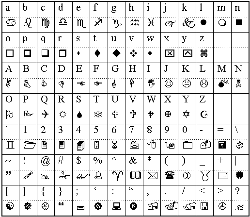
Due to its symbolic nature, interpreting Wingdings text programmatically poses a challenge, making it an interesting use case for custom OCR systems.
Dataset Creation
Since no existing dataset is available for Optical Character Recognition (OCR) in Wingdings font, we created one from scratch. The process involves generating images of words in the Wingdings font and mapping them to their corresponding English words.
To achieve this, we used the Wingdings Translator to convert English words into their Wingdings representations. For each converted word, an image was manually generated and stored in a folder named "wingdings_word_images".
Additionally, we create a "metadata.csv" file to maintain a structured record of the dataset along with the image path. This file contains two columns:
- Image Path: Specifies the file path for each image in the dataset.English Word: Lists the corresponding English word for each Wingdings representation.
The dataset can be downloaded from this link.
Preprocessing the Dataset
The images in the dataset vary in size due to the manual creation process. To ensure uniformity and compatibility with OCR models, we preprocess the images by resizing and padding them.
import pandas as pdimport numpy as npfrom PIL import Imageimport osfrom tqdm import tqdmdef pad_image(image, target_size=(224, 224)): """Pad image to target size while maintaining aspect ratio""" if image.mode != 'RGB': image = image.convert('RGB') # Get current size width, height = image.size # Calculate padding aspect_ratio = width / height if aspect_ratio > 1: # Width is larger new_width = target_size[0] new_height = int(new_width / aspect_ratio) else: # Height is larger new_height = target_size[1] new_width = int(new_height * aspect_ratio) # Resize image maintaining aspect ratio image = image.resize((new_width, new_height), Image.Resampling.LANCZOS) # Create new image with padding new_image = Image.new('RGB', target_size, (255, 255, 255)) # Paste resized image in center paste_x = (target_size[0] - new_width) // 2 paste_y = (target_size[1] - new_height) // 2 new_image.paste(image, (paste_x, paste_y)) return new_image# Read the metadatadf = pd.read_csv('metadata.csv')# Create output directory for processed imagesprocessed_dir = 'processed_images'os.makedirs(processed_dir, exist_ok=True)# Process each imagenew_paths = []for idx, row in tqdm(df.iterrows(), total=len(df), desc="Processing images"): # Load image img_path = row['image_path'] img = Image.open(img_path) # Pad image processed_img = pad_image(img) # Save processed image new_path = os.path.join(processeddir, f'processed{os.path.basename(img_path)}') processed_img.save(new_path) new_paths.append(new_path)# Update dataframe with new pathsdf['processed_image_path'] = new_pathsdf.to_csv('processed_metadata.csv', index=False)print("Image preprocessing completed!")print(f"Total images processed: {len(df)}")First, each image is resized to a fixed height while maintaining its aspect ratio to preserve the visual structure of the Wingdings characters. Next, we apply padding to make all images the same dimensions, typically a square shape, to fit the input requirements of neural networks. The padding is added symmetrically around the resized image, with the background color matching the original image's background.
Splitting the Dataset
The dataset is divided into three subsets: training (70%), validation (dev) (15%), and testing (15%). The training set is used to teach the model, the validation set helps fine-tune hyperparameters and monitor overfitting, and the test set evaluates the model’s performance on unseen data. This random split ensures each subset is diverse and representative, promoting effective generalization.
import pandas as pdfrom sklearn.model_selection import train_test_split# Read the processed metadatadf = pd.read_csv('processed_metadata.csv')# First split: train and temporarytrain_df, temp_df = train_test_split(df, train_size=0.7, random_state=42)# Second split: validation and test from temporaryval_df, test_df = train_test_split(temp_df, train_size=0.5, random_state=42)# Save splits to CSVtrain_df.to_csv('train.csv', index=False)val_df.to_csv('val.csv', index=False)test_df.to_csv('test.csv', index=False)print("Data split statistics:")print(f"Training samples: {len(train_df)}")print(f"Validation samples: {len(val_df)}")print(f"Test samples: {len(test_df)}")Visualizing the Dataset
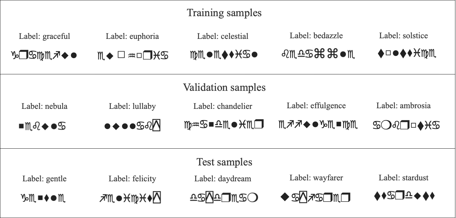
To better understand the dataset, we visualize samples from each split. Specifically, we display 5 examples from the training set, 5 from the validation set, and 5 from the test set. Each visualization includes the Wingdings text as an image alongside its corresponding label in English. This step provides a clear overview of the data distribution across the splits and ensures the correctness of the dataset mappings.
import matplotlib.pyplot as pltfrom PIL import Imageimport pandas as pddef plot_samples(df, num_samples=5, title="Sample Images"): # Set larger font sizes plt.rcParams.update({ 'font.size': 14, # Base font size 'axes.titlesize': 16, # Subplot title font size 'figure.titlesize': 20 # Main title font size }) fig, axes = plt.subplots(1, num_samples, figsize=(20, 4)) fig.suptitle(title, fontsize=20, y=1.05) # Randomly sample images sample_df = df.sample(n=numsamples) for idx, (, row) in enumerate(sample_df.iterrows()): img = Image.open(row['processed_image_path']) axes[idx].imshow(img) axes[idx].set_title(f"Label: {row['english_word_label']}", fontsize=16, pad=10) axes[idx].axis('off') plt.tight_layout() plt.show()# Load splitstrain_df = pd.read_csv('train.csv')val_df = pd.read_csv('val.csv')test_df = pd.read_csv('test.csv')# Plot samples from each splitplot_samples(train_df, title="Training Samples")plot_samples(val_df, title="Validation Samples")plot_samples(test_df, title="Test Samples")Samples from the data are visualised as:
Train an OCR Model
First we need to import the required libraries and dependencies:
import torchimport torch.nn as nnfrom torch.utils.data import Dataset, DataLoaderfrom transformers import VisionEncoderDecoderModel, ViTImageProcessor, AutoTokenizerfrom PIL import Imageimport pandas as pdfrom tqdm import tqdmModel Training with ViTSTR
We use a Vision Encoder-Decoder model, specifically ViTSTR (Vision Transformer for Scene Text Recognition). We fine-tune it for our Wingdings OCR task. The encoder processes the Wingdings text images using a ViT (Vision Transformer) backbone, while the decoder generates the corresponding English word labels.
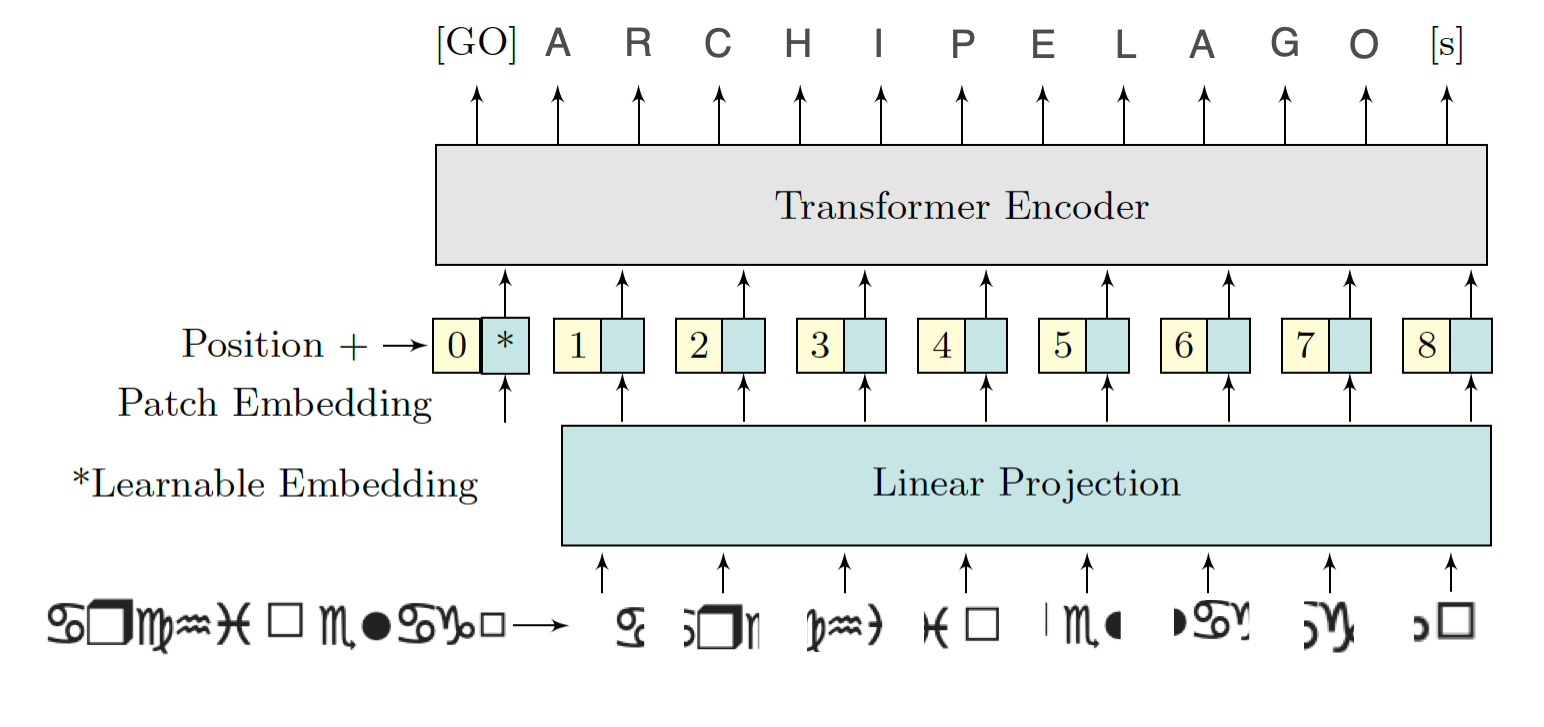
During training, the model learns to map pixel-level information from the images to meaningful English text. The training and validation losses are monitored to assess model performance, ensuring it generalizes well. After training, the fine-tuned model is saved for inference on unseen Wingdings text images. We use pre-trained components from Hugging Face for our OCR pipeline and fine tune them. The ViTImageProcessor prepares images for the Vision Transformer (ViT) encoder, while the bert-base-uncased tokenizer processes English text labels for the decoder. The VisionEncoderDecoderModel, combining a ViT encoder and GPT-2 decoder, is fine-tuned for image captioning tasks, making it ideal for learning the Wingdings-to-English mapping.
class WingdingsDataset(Dataset): def init(self, csv_path, processor, tokenizer): self.df = pd.read_csv(csv_path) self.processor = processor self.tokenizer = tokenizer def len(self): return len(self.df) def getitem(self, idx): row = self.df.iloc[idx] image = Image.open(row['processed_image_path']) label = row['english_word_label'] # Process image pixel_values = self.processor(image, return_tensors="pt").pixel_values # Process label encoding = self.tokenizer( label, padding="max_length", max_length=16, truncation=True, return_tensors="pt" ) return { 'pixel_values': pixel_values.squeeze(), 'labels': encoding.input_ids.squeeze(), 'text': label }def train_epoch(model, dataloader, optimizer, device): model.train() total_loss = 0 progress_bar = tqdm(dataloader, desc="Training") for batch in progress_bar: pixel_values = batch['pixel_values'].to(device) labels = batch['labels'].to(device) outputs = model(pixel_values=pixel_values, labels=labels) loss = outputs.loss optimizer.zero_grad() loss.backward() optimizer.step() total_loss += loss.item() progress_bar.set_postfix({'loss': loss.item()}) return total_loss / len(dataloader)def validate(model, dataloader, device): model.eval() total_loss = 0 with torch.no_grad(): for batch in tqdm(dataloader, desc="Validating"): pixel_values = batch['pixel_values'].to(device) labels = batch['labels'].to(device) outputs = model(pixel_values=pixel_values, labels=labels) loss = outputs.loss total_loss += loss.item() return total_loss / len(dataloader)# Initialize models and tokenizersprocessor = ViTImageProcessor.from_pretrained("google/vit-base-patch16-224-in21k")tokenizer = AutoTokenizer.from_pretrained("bert-base-uncased")model = VisionEncoderDecoderModel.from_pretrained("nlpconnect/vit-gpt2-image-captioning")# Create datasetstrain_dataset = WingdingsDataset('train.csv', processor, tokenizer)val_dataset = WingdingsDataset('val.csv', processor, tokenizer)# Create dataloaderstrain_loader = DataLoader(train_dataset, batch_size=32, shuffle=True)val_loader = DataLoader(val_dataset, batch_size=32)# Setup trainingdevice = torch.device('cuda' if torch.cuda.is_available() else 'cpu')model = model.to(device)optimizer = torch.optim.AdamW(model.parameters(), lr=5e-5)num_epochs = 20 #(change according to need)# Training loopfor epoch in range(num_epochs): print(f"\nEpoch {epoch+1}/{num_epochs}") train_loss = train_epoch(model, train_loader, optimizer, device) val_loss = validate(model, val_loader, device) print(f"Training Loss: {train_loss:.4f}") print(f"Validation Loss: {val_loss:.4f}")# Save the modelmodel.save_pretrained('wingdings_ocr_model')print("\nTraining completed and model saved!")The training is carried for 20 epochs in Google Colab. Although it gives fair result with 20 epochs, it's a hyper parameter and can be increased to attain better accuracy. Dropout, Image Augmentation and Batch Normalization are a few more hyper-parameters one can play with to ensure model is not overfitting. The training stats and the loss and accuracy curve for train and validation sets on first and last epochs are given below:
Epoch 1/20Training: 100%|██████████| 22/22 [00:36<00:00, 1.64s/it, loss=1.13]Validating: 100%|██████████| 5/5 [00:02<00:00, 1.71it/s]Training Loss: 2.2776Validation Loss: 1.0183........................................Epoch 20/20Training: 100%|██████████| 22/22 [00:35<00:00, 1.61s/it, loss=0.0316]Validating: 100%|██████████| 5/5 [00:02<00:00, 1.73it/s]Training Loss: 0.0246Validation Loss: 0.5970Training completed and model saved!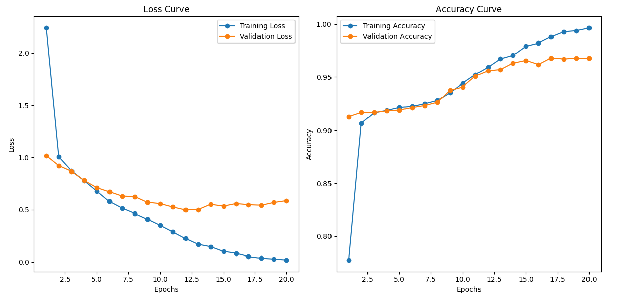
Using the Saved Model
Once the model has been trained and saved, you can easily load it for inference on new Wingdings images. The test.csv file created during preprocessing is used to create the test_dataset. Here’s the code to load the saved model and make predictions:
# Load the trained modelmodel = VisionEncoderDecoderModel.from_pretrained('wingdings_ocr_model')processor = ViTImageProcessor.from_pretrained("google/vit-base-patch16-224-in21k")tokenizer = AutoTokenizer.from_pretrained("bert-base-uncased")# Create test dataset and dataloadertest_dataset = WingdingsDataset('test.csv', processor, tokenizer)test_loader = DataLoader(test_dataset, batch_size=32)Model Evaluation
After training, we evaluate the model's performance on the test split to measure its performance. To gain insights into the model's performance, we randomly select 10 samples from the test split. For each sample, we display the true label (English word) alongside the model's prediction and check if they match.
import seaborn as snsimport matplotlib.pyplot as pltfrom PIL import Imagedef plot_prediction_samples(image_paths, true_labels, pred_labels, num_samples=10): # Set figure size and font sizes plt.rcParams.update({ 'font.size': 14, 'axes.titlesize': 18, 'figure.titlesize': 22 }) # Calculate grid dimensions num_rows = 2 num_cols = 5 num_samples = min(num_samples, len(image_paths)) # Create figure fig, axes = plt.subplots(num_rows, num_cols, figsize=(20, 8)) fig.suptitle('Sample Predictions from Test Set', fontsize=22, y=1.05) # Flatten axes for easier indexing axes_flat = axes.flatten() for i in range(num_samples): ax = axes_flat[i] # Load and display image img = Image.open(image_paths[i]) ax.imshow(img) # Create label text true_text = f"True: {true_labels[i]}" pred_text = f"Pred: {pred_labels[i]}" # Set color based on correctness color = 'green' if true_labels[i] == pred_labels[i] else 'red' # Add text above image ax.set_title(f"{true_text}\n{pred_text}", fontsize=14, color=color, pad=10, bbox=dict(facecolor='white', alpha=0.8, edgecolor='none', pad=3)) # Remove axes ax.axis('off') # Remove any empty subplots for i in range(num_samples, num_rows * num_cols): fig.delaxes(axes_flat[i]) plt.tight_layout() plt.show() # Evaluationdevice = torch.device('cuda' if torch.cuda.is_available() else 'cpu')model = model.to(device)model.eval()predictions = []ground_truth = []image_paths = []with torch.no_grad(): for batch in tqdm(test_loader, desc="Evaluating"): pixel_values = batch['pixel_values'].to(device) texts = batch['text'] outputs = model.generate(pixel_values) pred_texts = tokenizer.batch_decode(outputs, skip_special_tokens=True) predictions.extend(pred_texts) ground_truth.extend(texts) image_paths.extend([row['processed_imagepath'] for , row in test_dataset.df.iterrows()])# Calculate and print accuracyaccuracy = accuracy_score(ground_truth, predictions)print(f"\nTest Accuracy: {accuracy:.4f}")# Display sample predictions in gridprint("\nDisplaying sample predictions:")plot_prediction_samples(image_paths, ground_truth, predictions) The evaluation gives the following output:
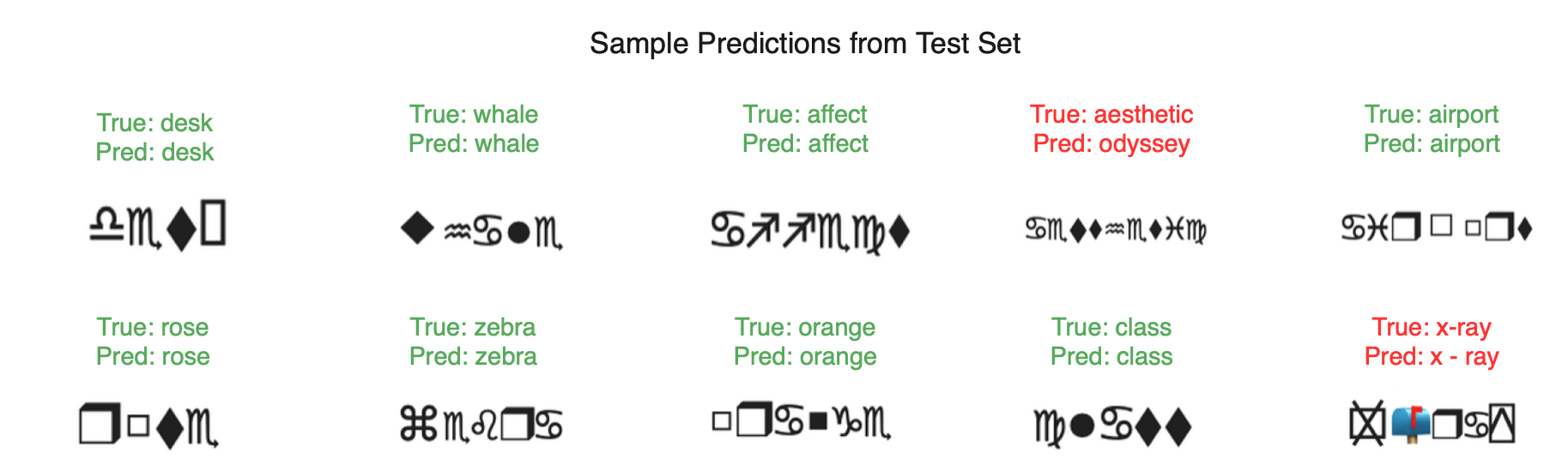
Analysing the output given by the model, we find that the predictions match the reference/original labels fairly well. Although the last prediction is correct it is displayed in red because of the spaces in the generated text.
All the code and dataset used above can be found in this Github repository. And the end to end training can be found in the following colab notebook
Discussion
When we see the outputs, it becomes clear that the model performs really well. The predicted labels are accurate, and the visual comparison with the true labels demonstrates the model's strong capability in recognizing the correct classes.
The model's excellent performance could be attributed to the robust architecture of the Vision Transformer for Scene Text Recognition (ViTSTR). ViTSTR stands out due to its ability to seamlessly combine the power of Vision Transformers (ViT) with language models for text recognition tasks.
A comparison could be made by experimenting with different ViT architecture sizes, such as varying the number of layers, embedding dimensions, or the number of attention heads. Models like ViT-Base, ViT-Large, and ViT-Huge can be tested, along with alternative architectures like:
- DeiT (Data-efficient Image Transformer)Swin Transformer
By evaluating these models of different scales, we can identify which architecture is the most efficient in terms of performance and computational resources. This will help determine the optimal model size that balances accuracy and efficiency for the given task.
For tasks like extracting information from documents, tools such as Nanonets’ Chat with PDF have evaluated and used several state of the LLMs along with custom in-house trained models and can offer a reliable way to interact with content, ensuring accurate data extraction without risk of misrepresentation.
